In the standard moral hazard framework of chapter 4, it was first assumed that the agent had no private information of his own. In insurance markets, insurees often have some prior information about how risky they are before exerting any effort to prevent this risk. Similarly, in credit markets, a borrower may know the average return of his project before exerting any effort and sharing the resulting profits with a lender. Those examples illustrate how frequent adverse selection and moral hazard are intertwined. A general formulation of these mixed models, where adverse selection takes place before moral hazard, would be cumbersome to present. However, a few dimensions of the analysis can already be singled out by studying some examples.
1. Random Surplus and Screening
In the pure adverse selection framework of chapter 2, the principal was able to verify and contract on all the agent’s actions. Of course, when moral hazard also occurs, this complete contractibility is no longer possible: some actions of the agent remain, by definition, under the agent’s sole control.
Consider a situation where moral hazard affects the random benefit that the principal draws from his relationship with the agent. In the mixed model we ana- lyze below, the principal already has a screening device at his disposal to start with. The random benefit Shqi he gets from dealing with the agent depends indeed on an observable, the agent’s production q, which can be used to screen the agent’s type.
Let us thus assume that, with probability π(e) (resp. 1 − π(e)) the benefit of production obtained by the principal is Sh(q) (resp. Sl(q) with Sh(q) > Sl(q), where the moral hazard variable e belongs to {0, 1}. Of course, we assume that Si(·), for i = h, l, is increasing and strictly concave (Si‘ > 0 and Si“ < 0) and satis- fies the Inada condition Si‘(0) = ∞. To motivate this random surplus model, one can think of effort as improving the quality of the product sold by the agent so that it generates a higher surplus. Of course, exerting effort will cost the agent a non- monetary disutility ψ(e) with the usual normalizations ψ(0) = 0 and ψ(1) = ψ. Moreover, the agent produces at a constant marginal cost r. As always, we assume that θ belongs to ![]() with respective probabilities v and 1 − v. For simplic-ity, we also assume that the agent is risk neutral and protected by limited liability.
with respective probabilities v and 1 − v. For simplic-ity, we also assume that the agent is risk neutral and protected by limited liability.
In this framework, the principal has two observables with which he can screen the agent’s efficiency parameter; in fact, this is a special case of the multi-output

Figure 7.1: Timing of Contracting with Adverse Selection Followed by Moral Hazard
framework studied in section 2.10. These two observables are first, whether the good sold has a high or a low quality and second, the amount of this good that is actually produced. Hence, the contract offered to the agent is a priori stochastic; the transfer received by the agent depends on the realized quality of the good.
The timing of contracting with adverse selection being followed by moral hazard is illustrated in figure 7.1.
Typically, a direct revelation mechanism is thus a menu of triplets ![]()
![]() stipulating the transfers th and tl made to the agent depending on the quality of the good and an output q as functions of the agent’s report on his type, θ˜. Moreover, we assume that contracting takes place at the interim stage (date t = 1), i.e., after the agent has learned his private information, but before the agent exerts effort.4 In what follows, we also assume that the principal finds it valuable to always induce a high level of effort from both types of agent. Using our usual notations, the efficient agent’s adverse selection incentive constraint is written as:
stipulating the transfers th and tl made to the agent depending on the quality of the good and an output q as functions of the agent’s report on his type, θ˜. Moreover, we assume that contracting takes place at the interim stage (date t = 1), i.e., after the agent has learned his private information, but before the agent exerts effort.4 In what follows, we also assume that the principal finds it valuable to always induce a high level of effort from both types of agent. Using our usual notations, the efficient agent’s adverse selection incentive constraint is written as:

with, in addition, the moral hazard incentive constraint
![]()
so that the efficient agent exerts a positive effort.
Similarly, the inefficient agent’s adverse selection incentive constraint becomes

and his moral hazard incentive constraint is
![]()
Since contracting takes place at the interim stage, the agent’s participation constraints are written as:
Finally, the following limited liability constraints must be satisfied. For the efficient type [(7.7), (7.8)] and for the inefficient type [(7.9), (7.10)]:

The number of constraints that we are facing to solve this problem is already huge, and our first goal should be to get rid of some of them. A preliminary remark is useful to simplify the analysis significantly. Indeed, focusing on cases where the limited liability constraints are binding for both types, note that both types must be given the same transfer differential th− tl to exert effort at a minimal cost for the principal, namely ![]() . Hence, at the optimum the incentive constraints (7.1) and (7.3) can be simplified to yield, respectively,
. Hence, at the optimum the incentive constraints (7.1) and (7.3) can be simplified to yield, respectively,
![]()
and
![]()
We let the reader check that the only relevant constraints are the adverse selection incentive compatibility constraint of an efficient type (7.11) and the lim- ited liability constraint of the inefficient type (7.10). When the expected payments to the agent ![]() in both states of nature are replaced by, respectively,
in both states of nature are replaced by, respectively, ![]() , the principal’s problem is then written as:
, the principal’s problem is then written as:

This optimization leads immediately to ![]() . Hence, we can compute the rent of each type of agent as, respectively,
. Hence, we can compute the rent of each type of agent as, respectively,
![]()
and
![]()
The reader will have recognized that these rents are precisely the informa-tion rents obtained under pure adverse selection (Δθq¯ and 0 respectively, as in chapter 2), added up with the limited liability rent obtained under pure moral haz- ard ( ![]() , as in chapter 4). In this simple model with a risk-neutral agent protected by limited liability constraints, the agent’s rent coming from the mixed model is simply obtained by adding up the respective rents due to adverse selection and moral hazard.
, as in chapter 4). In this simple model with a risk-neutral agent protected by limited liability constraints, the agent’s rent coming from the mixed model is simply obtained by adding up the respective rents due to adverse selection and moral hazard.
Solving for the optimal contract is now straightforward. The optimal outputs are obtained by equating expected marginal benefits and marginal virtual costs. For the efficient type, we find no output distortion as in a pure adverse selection model. Indeed, we have qSB = q∗, where the first-best production now takes into account the random nature of quality and is defined by
![]()
For the inefficient type, we have instead
![]()
The production of the inefficient type is distorted downward below the first-best output ![]() . As under pure adverse selection, this downward distortion helps to reduce the agent’s information rent coming from his private information on θ.
. As under pure adverse selection, this downward distortion helps to reduce the agent’s information rent coming from his private information on θ.
The reader might think that adding moral hazard in this model has no alloca- tive impact on the distortion due to adverse selection, which is exactly the same as if effort was observable. This is not completely true. Indeed, the output q¯SB is only the solution as long as shutdown of the least efficient type is not optimal. The no-shutdown condition is now written as

Simplifying, we find that the inefficient agent produces as long as the expected surplus he generates is greater than the sum of the adverse selection rent left to an efficient type and the limited liability rent left to the inefficient type. This condition is written as

With this condition, we see the role played by moral hazard in hardening the adverse selection problem. Inducing effort requires giving up a limited liability rent to the inefficient type. This rent plays exactly the same role as a fixed cost in a pure adverse selection framework (see section 2.6.3). It hardens the r¯-agent’s par- ticipation constraint and makes shutdown of the least efficient type more valuable for the principal. From this example, we can thus conclude that moral hazard hardens the adverse selection incentive problem. We state this as a general (but rather imprecise) proposition.
Proposition 7.1: In mixed models with adverse selection before moral haz- ard, preventing moral hazard hardens the adverse selection problem, and allocative distortions are greater than under pure adverse selection.
Laffont (1995) analyzes a related model of environmental regulation where Sl(q) = Sh(q) − d(q) and d(q) is an environmental damage.
The added complexity of his model comes from the fact that the disutility of effort depends directly on the level of production.
2. The Extended Revelation Principle
In section 7.1.1, we have studied a simple example, assuming a priori that the revelation principle holds in this context with both adverse selection and moral hazard. Now we will prove this principle, still using the basic structure of the model of section 7.1.1 for pedagogical purposes. The framework is nevertheless slightly more general, because we now allow the probability of having a high quality good to be a function of both the agent’s effort e and his type θ. This added complexity turns out to be a useful intermediate step before analyzing the more complex model of the insurance market covered in section 7.1.3.
Just as in section 2.9, let us first consider a general mechanism in this con- text. As usual, a mechanism stipulates a message space M and an outcome func-tion. Because the quality of the good is observed, that mechanism is a triplet ![]() stipulating a transfer for each quality and an output level as functions of the agent’s message m, which belongs to M.
stipulating a transfer for each quality and an output level as functions of the agent’s message m, which belongs to M.
Our goal is to show a revelation principle in such a context. In order to do so, we must first describe the agent’s behavior in front of any such mechanism. This description is more complex than in chapter 2. Indeed, given his type, the agent must now choose not only a message to be sent to the principal but also, given this message, what is the best effort that he should exert. Denoting by m∗(θ) and e∗(θ) the optimal message and effort, we have

Rewriting (7.18), we find

Just as in section 2.9, let us construct a direct revelation mechanism ![]()
![]() . We can now state our version of the revelation principle.
. We can now state our version of the revelation principle.
Proposition 7.2: There is no loss of generality in restricting the principal to offer a truthful direct revelation mechanism mthhr˜in tlhr˜in qhr˜ipr˜∈t and to recommend a choice of effort e∗hr˜i. With such a mechanism, the agent truthfully reveals his type to the principal and obeys the recommendation on the choice of effort.
Proof: The proof is straightforward and follows almost the same path as that of proposition 2.2. Using (7.19) and the definition of the direct revelation mechanism ![]() associated with any mechanism
associated with any mechanism ![]() , we have
, we have

This latter inequality being true for all m˜ , it is in particular true for ![]() for all θ˜ in Θ. Hence, we have
for all θ˜ in Θ. Hence, we have

This latter constraint means that the agent with type θ prefers to reveal his type to the principal and obey his recommendation on what should be the level of effort.
The revelation principle that we proved above has the same flavor as in a pure adverse selection framework. The logic is similar: the principal can always replicate the agent’s choices by incorporating the agent’s optimal message strategy into the initial contract he offers. However, on top of requesting that the agent sends a truthful message on his type, the principal also recommends now that the agent choose a particular level of effort.
Remark: Instead of insisting on the principal recommending a choice of effort to the agent, one could view this choice as being completely delegated and incorporated into the adverse selection problem in a way that affects the different parties’ utility functions. To see this point more precisely, let us define the agent’s indirect utility function UI(·) as

The revelation principle can be directly applied at this stage to get the following pure adverse selection incentive compatibility con- straints:

The difficulty for the modeller comes from the fact that these incentive compatibility constraints may not be as easily ordered as those of the pure adverse selection models in chapters 2 and 3. The indirect utility function UI(·) can fail to satisfy the Spence-Mirrlees property even in highly structured settings.
Myerson (1982) developed the extended revelation principal above in a more abstract setting. He used the expression obedience to char-acterize the fact that the agent must follow the principal’s instructions on his choice of effort.
3. Insurance Contracts with Adverse Selection and Moral Hazard
Insurance contracts are good examples of contracts designed to solve simultane- ously an adverse selection problem (how risky the agent is), and a moral hazard problem (how to induce enough safety care from the agent). We have already touched on the analysis of each of those two problems separately in chapters 3 and 4. This section is aimed at explaining how those two problems interact.
Remark In view of the analysis of section 7.1.1, with an insurance contract the principal now has only two instruments, namely different transfers depending on whether an accident occurs or not, to perform two tasks: incentivizing the agent to exert effort and inducing infor- mation revelation. This creates much of the complexity of this kind of model.
Let us assume that a monopoly insurer, the principal, offers an insurance contract to agents having an initial wealth w. By having an accident, an agent incurs a monetary loss of d. There is a continuum of mass one of agents who differ ex ante according to their risk type θ. To make things simpler, we assume that, for each agent, θ belongs to ![]() and that these types are independently drawn with respective probabilities 1 − v and v. Thus θ¯ (resp. θ) corresponds to a high (resp. low) risk for all levels of the moral hazard variable e. By exerting an effort e, an agent with type θ increases his probability π(θ, e) of not having an accident. We have thus πe(θ, e) < 0 and πe(θ, e) > 0 for all pairs (0, e). Moreover, for technical reasons, we will assume that
and that these types are independently drawn with respective probabilities 1 − v and v. Thus θ¯ (resp. θ) corresponds to a high (resp. low) risk for all levels of the moral hazard variable e. By exerting an effort e, an agent with type θ increases his probability π(θ, e) of not having an accident. We have thus πe(θ, e) < 0 and πe(θ, e) > 0 for all pairs (0, e). Moreover, for technical reasons, we will assume that ![]() . Of course, the agent suffers from a disutility ψ(e) when exerting an effort. As usual, we assume that effort belongs to m0n 1p, with ψ(1) = ψ and ψ(0) = 0.
. Of course, the agent suffers from a disutility ψ(e) when exerting an effort. As usual, we assume that effort belongs to m0n 1p, with ψ(1) = ψ and ψ(0) = 0.
The insurance company requests a payment tn from the agent when no acci- dent occurs and gives a transfer ta in the case of an accident. Its objective function is thus V = π(θ, e)tn − (1 − π(θ, e))ta. With these specifications, an agent with type r who exerts effort e gets an expected utility U = π(θ, e)u(w − d + ta )- ψ(e), where u(·) is the agent’s Von Neuman-Morgenstern utility function defined on monetary gains (u‘ > 0 and u“ < 0).
With our usual notations, a direct revelation mechanism writes as a pair ![]() .
.
Let us also assume that the damage d is large enough. The benefits of avoiding a damage are then so large that inducing the high level of effort is always optimal for the insurance company. When he exerts a high effort and truthfully reports his type to the principal, the high-risk agent gets an expected utility
![]()
Similarly, the low-risk agent gets
![]()
Inducing both types to participate in this contract requires that the following participation constraints are satisfied:
![]()
and
![]()
To simplify the analysis, we also assume that
![]()
where Δπ(θ) = π(θ,1) − π(θ,0). This assumption simply means that both types are willing to exert a positive effort in the absence of any insurance contract. In this case, the right-hand sides of (7.26) and (7.27) are respectively given by ![]()
![]() . Note that we have U0 > U0¯, because
. Note that we have U0 > U0¯, because ![]() and u(w) > u(w − d).
and u(w) > u(w − d).
Because of moral hazard, inducing effort by both types calls for having the following moral hazard incentive constraints satisfied when agents report their types truthfully to the principal. For a high-risk agent, we get
![]()
For a low-risk agent, we have
![]()
Truthful revelation is obtained when the following adverse selection incentive constraints are satisfied: for the high-risk agent,
![]()
and for the low-risk agent,
![]()
Remark: As for (7.1) and (7.3), the complexity of the latter two incen- tive constraints already shows some of the technical difficulties faced by the economist in modelling mixed environments. Indeed, when he considers deviating along the adverse selection dimension and not telling the truth to the principal anymore, the agent may also choose to change his supply of effort. Even if inducing a high effort is optimal for the principal when both types tell the truth, it is not necessary for the mechanism to require an agent to continue to exert this high effort if the agent lies about his type. Even in this simple environment, the right-hand sides of (7.31) and (7.32) are hard to describe, because the values of these maximands depend on how an agent with a given risk type changes his effort supply when he chooses different insurance contracts.
To simplify this problem, let us assume that effort increases the probability that no accident occurs more when the agent is high risk than when he is low risk. This means that the following condition must be satisfied:
![]()
This condition ensures that the moral hazard incentive constraint for a high- risk type (7.29) is easier to satisfy than the one associated with a low-risk type (7.30). In this case, inducing effort from the low-risk agent requires a wedge between u(w − tn) and u(w − d + ta) that is large enough to ensure that a high-risk agent also prefers to exert a high effort, even when he lies and mimics a low-risk agent. Indeed, we have ![]() . This condition greatly simplifies the writing of the adverse selection incentive constraint for the high-risk agent, which now becomes
. This condition greatly simplifies the writing of the adverse selection incentive constraint for the high-risk agent, which now becomes
![]()
Let us now introduce a new set of variables:![]()
![]() . These new variables will help us describe the set of relevant constraints in a simpler way. As usual, we denote the inverse function of uh·i by h = u−1. Using these new variables, the expected profit of the insurance company is written as
. These new variables will help us describe the set of relevant constraints in a simpler way. As usual, we denote the inverse function of uh·i by h = u−1. Using these new variables, the expected profit of the insurance company is written as

The high-risk agent’s adverse selection incentive constraint (7.34) now becomes
![]()
The high-risk agent’s moral hazard incentive constraint is
![]()
The low-risk agent’s moral hazard incentive constraint is written as
![]()
Finally, the low-risk agent’s participation constraint can be expressed as
![]()
Neglecting the other constraints, which will be checked only ex post, the insurance company’s problem is written as

Before solving this problem it is useful to recall the main features of the optimal contracts found in the case of pure adverse selection and pure moral hazard.
In figure 7.2, we have represented the indifference curves of the high- and low-risk agents when they are forced to exert a positive effort, and this effort can be verified by a court of law. The indifference curve of the agent with a low probability of accident has a smaller slope than the indifference curve of an agent with a high probability of accident.
As we have shown in section 3.3.2, if r were perfectly known by the principal the agent would receive the full insurance contracts A∗ and B∗. Under pure adverse selection, however, the high-risk agent still receives full insurance at point BAS, but the low-risk agent receives contract AAS and is now imperfectly insured. Moving slightly away from A∗ to AAS entails only a second-order loss on the profit made by the principal with the low-risk agent, because the latter is then subject only to a small amount of risk. However, moving from A∗ to AAS also allows the principal to reduce the information rent of the high-risk agent to the first order.

Figure 7.2: Insurance Contracts: The Case of Pure Adverse Selection
Let us now turn to the case of pure moral hazard where effort is nonobservable but the agent’s type is perfectly known to the insurance company. The indifference curves of the different types now have a kink where the agent is indifferent between exerting effort or not. Note that the assumption π(θ, 1) > π(θ, 0) for each type θ implies that the indifference curve of each type has a smaller slope (in absolute value) when the agent exerts a positive effort than when he does not. Moreover, since we have assumed that ![]() , the indifference curves of the two different types can only cross each other once. The analysis of chapter 4 has shown us that the insurance company would like to offer contracts AMH or BMH to the agent, depending on his observable type, if the only issue was moral hazard. Each of these contracts is lying on an indifference curve where a given type of agent is exactly indifferent between exerting effort or not. Of course, these contracts are above the 45° line to induce effort. Therefore, they provide only partial insurance to the agent, whatever his type (figure 7.3).
, the indifference curves of the two different types can only cross each other once. The analysis of chapter 4 has shown us that the insurance company would like to offer contracts AMH or BMH to the agent, depending on his observable type, if the only issue was moral hazard. Each of these contracts is lying on an indifference curve where a given type of agent is exactly indifferent between exerting effort or not. Of course, these contracts are above the 45° line to induce effort. Therefore, they provide only partial insurance to the agent, whatever his type (figure 7.3).

Figure 7.3: Insurance Contracts: The Case of Pure Moral Hazard
Under pure moral hazard, we could replicate the analysis of chapter 4, taking into account that an agent with type r has a nonzero reservation utility given
by U0 , to show that point AMH corresponds to the ex post utility levels ![]()
![]() . Similarly, taking into account that a θ¯-agent has a nonzero reservation utility given by U0¯, point BMH corresponds to the ex post utility levels
. Similarly, taking into account that a θ¯-agent has a nonzero reservation utility given by U0¯, point BMH corresponds to the ex post utility levels ![]() .
.
Let us finally consider the more complex case entailing both moral hazard and adverse selection. Graphically, we see that the menu of contracts (AMH, BMH) is no longer incentive compatible. Following the logic of the case with pure adverse selection, the high-risk agent also would like to choose contract AMH in order to increase his expected utility. The new level of utility that can be achieved by doing so is obtained by moving up the indifference curve of a θ¯-agent in a northeast direction until it reaches point AMH.
More formally, the high-risk agent wants to mimic the low-risk one and exert a positive effort when

This latter inequality is satisfied when

which is true when assumption (7.28) holds.
To prevent the high-risk agent from lying, the principal offers the pair of con- tracts (ASB, BSB) described in figure 7.4. Following the logic of the model with pure adverse selection, the contract ASB offered to the low-risk agent entails more risk than under pure moral hazard to reduce the costly information rent of the high- risk type. Graphically, the indifference curve of a θ¯-agent crosses the indifference curve of a θ-agent at a point ASB on the northwest of point AMH. The high-risk agent is indifferent between contracts ASB and BMH, and the low-risk agent strictly prefers ASB to BMH. Contract ASB entails imperfect insurance to induce this type to exert an effort. It corresponds to an expected utility greater than U0¯, to reward the high-risk agent for having revealed his information. Importantly, and contrary to the case of pure adverse selection, by moving from BMH to BSB the principal no longer suffers from a second-order loss in profit but instead suffers from a first-order loss. In order to solve the moral hazard, the low-risk agent must bear a strictly positive amount of risk. Hence, AMH is no longer on the full insurance line but is now strictly above it. Starting from such a point, and increasing the risk to move towards ASB, will thus create a first-order loss of profit for the insurance company. Although ASB lies strictly above the low-risk agent’s moral hazard incentive constraint, it is nevertheless affected by moral hazard. Because of moral hazard, the high-risk agent must bear some risk. This risk affects the cost of his informa- tion rent from the principal’s point of view and makes it more costly. This cost increase in turn has an impact on the risk borne by the low-risk agent to reduce this rent.
To see more precisely how the low-risk agent’s risk is affected by the cost increase, note first that the participation constraint (7.26) is slack. Second, the

Figure 7.4: Insurance Contracts: Adverse Selection and Moral Hazard
adverse selection incentive compatibility constraint (7.37), the moral hazard incen- tive constraint in (7.38), and the participation constraint of the low-risk agent (7.40) are all binding at the solution to (P)i. This yields the following expressions of the second-best utilities of each type of agent in each state of nature:

where the dependence of those variables on Δu = un − ua, the risk borne by the low-risk agent, is explicit.
Inserting these expressions into the principal’s objective function yields a new problem, which depends only on Δu:

where (7.46) is the low-risk agent’s moral hazard incentive constraint.
We assume that the latter constraint is slack at the optimum, so that optimiz- ing with respect to Δu yields the following first-order condition, which implicitly defines ΔuSB as
Because π(θ, 1) > π(θ¯, 1), the right-hand side above is positive, and we conclude that ![]() . Hence, the low-risk agent must bear some risk, as in the case of pure adverse selection.
. Hence, the low-risk agent must bear some risk, as in the case of pure adverse selection.
We leave it to the reader to check that, to ensure that the moral hazard incentive constraint (7.46) is slack, a sufficient condition is that ![]()
![]() satisfy
satisfy

where we note that ![]()
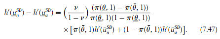
Note that, when h‘(.) is convex, Jensen’s inequality implies that the brack-eted term on the right-hand side of (7.47) is greater than ![]()
![]() . Hence, we have
. Hence, we have

Using the same techniques as in section 3.3.2, one can check that, with pure adverse selection, the insurance company would choose to let the low-risk agent bear a positive risk ![]() , such that
, such that
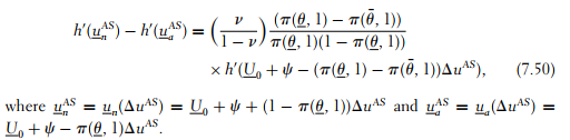
Under pure adverse selection, the principal’s objective function is concave with respect to Δu. Hence, the derivative of this objective function, which is proportional to

is decreasing in wu. Using (7.49) and (7.50), it can immediately be concluded that ΔuSB > ΔuAS.
With adverse selection and moral hazard, the risk borne by the low-risk agent is greater than with pure adverse selection. The intuition behind this result is straightforward. The high-risk agent must bear some risk to exert an effort, as can easily be seen by comparing un¯SB and ua¯SB. From the insurance company’s point of view, dealing with a high-risk agent now costs ![]()
![]() . The marginal cost of decreasing the risk Δu borne by the low-risk agent is thus
. The marginal cost of decreasing the risk Δu borne by the low-risk agent is thus ![]() . Taking into account the fact that
. Taking into account the fact that ![]() , this marginal cost is equal to
, this marginal cost is equal to ![]()
![]() , which is greater than
, which is greater than ![]()
![]() when h‘(·) is convex. Note that
when h‘(·) is convex. Note that ![]()
![]() represents exactly the marginal cost of decreasing the risk borne by the low-risk agent under pure adverse selection. Hence, the random- ness in the high-risk agent’s payoff, which is implied by moral hazard, makes the insurance company less eager to decrease the risk borne by the low-risk agent even more than under pure adverse selection. Point ASB lies on the north-west of AAS on the indifference curve of the low-risk agent that corresponds to his expected utility without any insurance U0.
represents exactly the marginal cost of decreasing the risk borne by the low-risk agent under pure adverse selection. Hence, the random- ness in the high-risk agent’s payoff, which is implied by moral hazard, makes the insurance company less eager to decrease the risk borne by the low-risk agent even more than under pure adverse selection. Point ASB lies on the north-west of AAS on the indifference curve of the low-risk agent that corresponds to his expected utility without any insurance U0.
Putting together our findings here with those of section 7.1.1, we can finally conclude that the agency costs of adverse selection and moral hazard are not simply added together as in proposition 7.1 but may sometimes strongly reinforce each other.
4. Models with “False Moral Hazard”
Another important class of mixed models that has received much attention in the literature actually entails no randomness at all in the benefit obtained by the principal when dealing with the agent. The link between effort, types, and the contractual variable available to the principal is thus completely deterministic. The difficulty of such models comes only from the fact that the observation of this variable does not allow the principal to perfectly disentangle the type of the agent and his level of effort. Typically, q is the observable and Q(·) is a deterministic mapping between type and effort pairs into the set of feasible observables, so that we have q = Q(θ, e). Hence, given a target value of q, which can be imposed by the principal, and given the agent’s type, effort is completely determined by the condition e = E(θ, q), where E(·) is implicitly defined by the identity q = Q(θ, E(θ, q)) for all θ in Θ and all q.
Those models can be classified under the name of false moral hazard, because the agent has no real freedom in choosing his effort level when he has decided how much to produce. This lack of freedom makes the analysis of these models closely related to the analysis of models with pure adverse selection that were seen in chapter 2. In order to illustrate false moral hazard, we present two models of procurement and optimal taxation that have been extensively used in the literature.
Example 1: The Procurement Model
Let us assume that the principal requests only one unit of good (q in {0, 1}) from the agent, yielding a gross surplus S. The cost of producing this unit is assumed to be observable. Had we kept the usual specification C(θ, q) = θq, with θ being dis- tributed in ![]() according to the common knowledge distribution (v, 1 − v) the knowledge of C = C(θ, 1) would give to the principal complete information on θ. To avoid this indirect finding of the efficiency parameter θ, let us assume that the cost of producing one unit of the good is not only related to the efficiency parameter θ but also to the agent’s effort e in an additive manner: C(θ, e) = θ − e. By exerting effort e, the agent reduces the cost of producing the good. The point is that the observation of the cost C = θ − e is not enough to infer perfectly the agent’s productivity parameter. Intuitively, an efficient agent θ can exert an effort e − Δθ and still produce at the same cost as a less efficient agent θ¯ exerting also effort e.
according to the common knowledge distribution (v, 1 − v) the knowledge of C = C(θ, 1) would give to the principal complete information on θ. To avoid this indirect finding of the efficiency parameter θ, let us assume that the cost of producing one unit of the good is not only related to the efficiency parameter θ but also to the agent’s effort e in an additive manner: C(θ, e) = θ − e. By exerting effort e, the agent reduces the cost of producing the good. The point is that the observation of the cost C = θ − e is not enough to infer perfectly the agent’s productivity parameter. Intuitively, an efficient agent θ can exert an effort e − Δθ and still produce at the same cost as a less efficient agent θ¯ exerting also effort e.
Let us denote by t the transfer received by the agent. Since cost is observable, it is an accounting convention to have this transfer being net of cost. The princi- pal’s profit is written as V = S − t − C. The agent’s utility becomes U = t − ψ(e), where ψ(·) is the disutility of effort, such that ψ’ > 0, ψ“ > 0 and ψ“‘ > 0. Expressed only in terms of observables, the agent’s utility can finally be written as U = t − ψ( θ − C).
The reader will have recognized a pure adverse selection model with the observable being the cost C. In this context, the revelation principle tells us that there is no loss of generality in restricting the principal to offer direct revelation mechanisms ![]() , which are truth-telling.
, which are truth-telling.
With our usual notations, the following incentive constraints have to be sat- isfied:

where, from the assumptions made on ![]() is decreas- ing and convex in C. Also, the participation constraints are
is decreas- ing and convex in C. Also, the participation constraints are

Note that the indifference curves of both types in the space (t, C) satisfy the single-crossing property with those of the efficient type having a smaller slope. The reader will have recognized the Spence-Mirrlees property, which allows us to conclude that, at the optimal contract, the relevant binding constraints are (7.51) and (7.54). The principal’s problem is thus written as

Both constraints above are binding at the optimum, and we have thus U SB = Ф(C¯SB) and U¯SB = 0.
Optimizing with respect to the cost targets C and C¯ amounts to optimizing with respect to the effort levels e and e¯, which are indirectly requested from, respectively, an efficient type and an inefficient type once one has recognized that those cost targets and efforts are linked by the relationships C = θ − e and C¯ = θ¯ − e¯. Expressing the principal’s objective function in terms of efforts and taking into account that (7.51) and (7.54) are both binding at the optimum, the principal’s problem becomes

Optimizing with respect to e and e¯ yields, respectively,
![]()
and
![]()
Note that under complete information, both types would be asked to exert the same first-best level of effort e∗ such that the marginal disutility of effort equals the marginal cost reduction, i.e., ψ‘(e∗) = 1. Under asymmetric information, only the most efficient type continues to exert this first-best level of effort. In order to reduce the costly information rent of this efficient type, the effort of the less effi- cient type is reduced below the first-best, and e¯SB < e∗.
These results are not surprising in light of the analysis presented in chapter 2. However, here the novelty comes from the interpretation of the model. Because the efficient agent is residual claimant for his effort, we will say that he is put on a high-powered incentive scheme, which is akin to a fixed-fee contract. The inefficient agent under-supplies effort because he is only partially residual claimant for his effort. We will say that he is instead put on a low-powered incentive scheme, which is closer to a cost-plus contract.
To better understand these denominations, let us assume that the princi- pal offers a nonlinear contract T hCi, which is defined over all C in [0, +∞].
This mechanism should implement precisely the second-best allocation computed above, when the agent finds it optimal to exert effort eSB and e¯SB. Assuming dif-ferentiability of the schedule T (C) at the points CSB and C¯SB, we must have ![]() . Iden- tifying with (7.55) and (7.56), we find that T ‘(CSB) = 1 and T ‘(C¯SB) < 1. This shows that only the efficient agent is given full incentives in cost reduction. The inefficient agent gets only a function of his marginal effort in cost reduction and thus under-provides effort.
. Iden- tifying with (7.55) and (7.56), we find that T ‘(CSB) = 1 and T ‘(C¯SB) < 1. This shows that only the efficient agent is given full incentives in cost reduction. The inefficient agent gets only a function of his marginal effort in cost reduction and thus under-provides effort.
Let us now turn to the shape of the nonlinear schedule T hCi. To get some ideas on this shape, it is useful to look at figure 7.5.
To ensure that the agent, whatever his type, chooses the second-best cost target computed by the principal, it is enough that the nonlinear transfer T(C) be tangent to each indifference curve at points A and B. We may thus define T(C) as

Remark: In the case of a continuum of types, we will see in sec- tion 9.5.1 that the optimal contract can sometimes be implemented through a menu of linear contracts under rather weak assump- tions.
This procurement model is due to Laffont and Tirole (1986, 1993), who have built a whole theory of regulation and procurement with elements of both moral hazard and adverse selection. Interesting issues arise in the case where output is no longer zero or one, as in this model. Indeed, on top of cost, output can then also be used as a screening variable. Depending
on the exact mapping between cost, output, effort, and types, the pricing rule may or may not be distorted under asymmetric information. When it is not, Laffont and Tirole (1993) argue that there is a dichotomy between the pricing rule and the provision of incentives. Lazear (2000) uses a model with false moral hazard to analyze the relation between performance pay and productivity empirically. Lazear (2000) concludes: “workers respond to prices just as economic theory predicts.”

Figure 7.5: Implementation with a Nonlinear Schedule T(C)
Example 2: The Income Taxation Model
Let us now return to the optimal redistribution model studied in section 3.7. One weakness of that model was the fact that the government was assumed to be unable to observe the actual income of each agent. Standard taxation models relax this somewhat unrealistic assumption. In order to still have a meaningful informational problem, we must now assume that each agent produces an amount q = θe when his productivity parameter is θ (θ belongs to ![]() ) with respective probabilities 1 − v and v, and his effort e belongs to [0, e¯]. Effort costs the agent a disutility ψ(e) with ψ‘ > 0, ψ“ > 0 and ψ“‘ > 0 as before.
) with respective probabilities 1 − v and v, and his effort e belongs to [0, e¯]. Effort costs the agent a disutility ψ(e) with ψ‘ > 0, ψ“ > 0 and ψ“‘ > 0 as before.
Normalizing the price of the production good at one, q also represents the agent’s income, which is now assumed to be observable by the government. Note the similarity of this model with the procurement model above. Instead of being blended additively, type and effort are now blended multiplicatively into the observ- able that is available to the principal. When exerting effort e and paying a tax τ, the agent with productivity θ gets a utility U = q − τ− ψ(e), or, replacing effort as a function of the agent’s type and his income, ![]() . Again, the reader will have recognized that we are now back to a pure adverse selection model. In this context, a taxation mechanism can be viewed as a menu
. Again, the reader will have recognized that we are now back to a pure adverse selection model. In this context, a taxation mechanism can be viewed as a menu ![]() , where q is the agent’s revenue and τ is the corresponding tax payment. The incentive compatibility constraints for this model are written as
, where q is the agent’s revenue and τ is the corresponding tax payment. The incentive compatibility constraints for this model are written as
![]()
and
![]()
where ![]() is increasing and convex in q from the assumptions made on ψ(·) , (Φ’ > 0, Φ” > 0).
is increasing and convex in q from the assumptions made on ψ(·) , (Φ’ > 0, Φ” > 0).
On top of these incentive constraints, a taxation scheme is feasible if it satis-fies the government budget constraint ![]() . Expressing taxes as a function of the rents U¯ and U and efforts e¯ and e, this budget constraint becomes
. Expressing taxes as a function of the rents U¯ and U and efforts e¯ and e, this budget constraint becomes
![]()
The government wants to maximize the social welfare function vG(U¯) + (1 − v)G(U ), where G(·) is increasing and concave, (G‘ > 0 and G“ < 0). The principal’s problem is thus

We let the reader check that the relevant incentive constraint is, as usual, that of the most productive type θ¯. Denoting the multiplier of the budget constraint (7.59) by µ and the multiplier of the incentive constraint (7.57) by λ, we can write the Lagrangian of the problem as

where ![]() is increasing and convex in e. Optimizing with respect to U¯ and U yields, respectively,
is increasing and convex in e. Optimizing with respect to U¯ and U yields, respectively,

Summing (7.61) and (7.62), we obtain
![]()
and thus the budget constraint (7.59) is binding. Inserting this value of µ into (7.61), we get:
![]()
Because U¯SB > USB is necessary to satisfy the incentive constraint (7.57), and because G(·) is concave, we have λ > 0. Hence, the incentive constraint (7.57) is also binding.
Optimizing with respect to efforts, we immediately find that
![]()
and

In the complete information framework, the government could perfectly redis- tribute wealth between both groups of agents to equalize their utilities. Moreover, the government could recommend to exert first-best efforts e¯* and e∗ such that the marginal disutility of effort of each type would equal his productivity, i.e., ![]() .
.
Under asymmetric information, only the most productive agent still exerts the first-best level of effort. Inducing information revelation calls for creating a positive wedge between the utilities of the high- and the low-productivity agents. Because the principal is adverse to inequality in the distribution of utilities, this risk is socially costly. To reduce this cost, the principal reduces the low-productivity agent’s effort below its first-best value and eSB < e∗.
Interestingly, it is worthwhile to recast these results in terms of the progressive-ness or lack of progressiveness of the tax schedule. Indeed, as in the procurement model above, let us think of this optimal allocation as being implemented by a nonlinear income tax m•hqip. When he faces this nonlinear tax, the high- (resp. low-) productivity agent will choose to exert the second best level of efforts e¯SB and eSB, such that ![]() . Using (7.65) and (7.66), the marginal tax rates that concern each type are thus τ‘(q¯) = 0 and τ‘(q) > 0. Hence, the high-productivity agent is not taxed at the margin. The marginal tax rate at the top of the distribution is zero. The low-productivity agent instead has a positive marginal tax rate. The optimal taxation scheme is thus regressive at the margin, a surprising feature that has generated much debate in the optimal taxation literature.
. Using (7.65) and (7.66), the marginal tax rates that concern each type are thus τ‘(q¯) = 0 and τ‘(q) > 0. Hence, the high-productivity agent is not taxed at the margin. The marginal tax rate at the top of the distribution is zero. The low-productivity agent instead has a positive marginal tax rate. The optimal taxation scheme is thus regressive at the margin, a surprising feature that has generated much debate in the optimal taxation literature.
The basic model above is based on Diamond (1998a), who simplifies the initial framework of Mirrlees (1971) by restricting the analysis to quasi-linear utility functions.
Source: Laffont Jean-Jacques, Martimort David (2002), The Theory of Incentives: The Principal-Agent Model, Princeton University Press.