Consider the twice repetition of the model in chapter 2, where we can make various assumptions on the information structure and, in particular, on how it evolves over time. The goal of this section is to compare the optimal long-term contract with its static counterpart.
1. Perfect Correlation of Types and Risk Neutrality
Let us first start with the simplest case, where the adverse selection parameter θ in ![]() is the same in both periods. The principal’s objective function writes now as
is the same in both periods. The principal’s objective function writes now as ![]() , where qi (resp. ti) is output (resp. transfer) at date t = i. The discount factor is δ≥ 0, and we can allow it to be greater than one to represent cases where period 2 lasts much longer than period 1. The risk-neutral agent has the same discount factor as the principal and, because of perfect correlation of types between both periods, his objective function is written as
, where qi (resp. ti) is output (resp. transfer) at date t = i. The discount factor is δ≥ 0, and we can allow it to be greater than one to represent cases where period 2 lasts much longer than period 1. The risk-neutral agent has the same discount factor as the principal and, because of perfect correlation of types between both periods, his objective function is written as ![]() .
.

Figure 8.1: Timing of Contracting with Adverse Selection and Perfect Correlation
Note that the principal controls a pair of actions performed by the agent: the agent’s productions at each date. Thus we are in a special case of the multi-output regulation studied in section 2.10, with the agent and the principal’s objective functions being additively separable over the two periods.
The timing of contracting is described in figure 8.1.
With full generality, a long-term contract stipulates transfers and quantities in each period as a function of the whole past history of the game up to that period. In the case of two periods, this means that a typical long-term contract writes as a pair of nonlinear transfers ![]() dependent, at each period, on the current as well as the past output realizations.
dependent, at each period, on the current as well as the past output realizations.
Since the principal can commit intertemporally, the revelation principle remains valid in this intertemporal framework, and the pair of nonlinear transfers described above can be replaced by a truthful direct revelation mechanism. With such a mechanism, the agent reports his type to the principal at a date t = 0.75, just before outputs and transfers for the first period are implemented. Moreover, because of risk neutrality, only the aggregate transfer t = t1 + δt2 matters when describing both the agent and the principal’s utility functions. In this framework, a direct revelation mechanism is thus a pair of triplets ![]() , stipulating an aggregate transfer and an output target for each date according to the firm’s report on the agent’s type.
, stipulating an aggregate transfer and an output target for each date according to the firm’s report on the agent’s type.
Denoting the efficient and the inefficient agents’ information rents over both periods by, respectively, ![]() the following incentive constraints must be satisfied:
the following incentive constraints must be satisfied:
![]()
and

The intertemporal participation constraints of both types are, respectively,
![]()
and
![]()
Remark: Note that these participation constraints stipulate that only the agent’s intertemporal rent must be positive. So, we assume momen- tarily that the agent commits to stay in the relationship once he has accepted the contract at date t = 0.5. In period 1, the agent can make a loss if it is covered by a gain in period 2, and vice versa.
The principal’s problem becomes

Of course, the relevant constraints are, again, the efficient type’s incentive constraint in (8.1) and the inefficient type’s participation constraint in (8.4). For the optimal dynamic contract, only the efficient type gets a positive intertemporal rent, which is worth ![]() , and the inefficient type’s participation constraint is binding so that U¯ = 0. Inserting these expressions of the intertemporal rents into the principal’s objective function and optimizing with respect to outputs, we immediately get the following proposition where we index this solution with a superscript D, meaning dynamics.
, and the inefficient type’s participation constraint is binding so that U¯ = 0. Inserting these expressions of the intertemporal rents into the principal’s objective function and optimizing with respect to outputs, we immediately get the following proposition where we index this solution with a superscript D, meaning dynamics.
Proposition 8.1: With perfectly correlated types and a risk-neutral agent, the optimal long-term contract with full commitment for two periods is twice the repetition of the optimal static contract.
- The constraints in (8.1) and (8.4) are the only binding ones.
- The efficient agent produces efficiently in both periods
 such that .
- The inefficient agent produces less than the first-best output in both periods , such that:
![]()
It is the same output as in the optimal static contract q¯D = q¯SB.
- Only the efficient agent gets a positive intertemporal rent .
Remark 1: Even if the optimal long-term contract implements the same outputs levels and the same intertemporal rents as the opti- mal static contract of chapter 2 repeated twice, some indeterminacy remains concerning the intertemporal distribution of these rents, because only the intertemporal transfers are pinned down by the binding constraints in (8.1) and (8.4).
Remark 2: Let us instead assume that the principal offers the agent a contract covering both periods at the ex ante stage, i.e., before the agent learns his private information. Moreover, let us consider the case where the agent has an infinite degree of risk aversion below zero wealth and a positive degree above. In that case, the agent’s intertem- poral participation constraints in (8.3) and (8.4) should be replaced by a pair of participation constraints for each period, namely ![]()
![]()
![]() , respectively. Under these assumptions, the same result as in proposition 8.1 still holds. Moreover, because the agent has a positive rent in any given period, there is no need for him to commit to stay in the relationship. The agent never has the incentive to renege on the long-term contract offered by the principal. The main differ- ence between the case of risk neutrality and interim contracting is that the intertemporal distribution of rents is now completely defined. The efficient type gets a positive rent in both periods
, respectively. Under these assumptions, the same result as in proposition 8.1 still holds. Moreover, because the agent has a positive rent in any given period, there is no need for him to commit to stay in the relationship. The agent never has the incentive to renege on the long-term contract offered by the principal. The main differ- ence between the case of risk neutrality and interim contracting is that the intertemporal distribution of rents is now completely defined. The efficient type gets a positive rent in both periods ![]() , for i = 1, 2. The inefficient type instead gets zero in both periods.
, for i = 1, 2. The inefficient type instead gets zero in both periods.
Remark 3: Of course, the optimal long-term contract would not be the twice replica of the one-shot optimal contract if either the agent’s cost function or the principal’s value functions were not separable over the two periods.
Remark 4: Importantly, proposition 8.1 shows the importance of the principal’s ability to commit. If the firm is inefficient, this fact is now common knowledge at the beginning of period 2. Still, the principal implements an inefficient contract with under-production. We come back to this commitment issue in section 8.1.4 below.
The dynamics of the optimal contract with full commitment was first analyzed in different settings by Roberts (1983) and Baron and Besanko(1984b). At a more abstract level, the applicability of the revelation principle to a dynamic context (with possibly more complex information structures than those with perfect correlation) was demonstrated by Myerson (1986) and Forges (1986) (see Myerson 1991 for a review of the argument).
2. Independent Types and Risk Neutrality
Let us now turn to the case where the agent’s marginal cost in periods 1 and 2 are independently drawn from the same support ![]() , with identical probabilities ν and 1 − ν. The risk-neutral agent’s utility is written as
, with identical probabilities ν and 1 − ν. The risk-neutral agent’s utility is written as ![]()
![]() , where θi is his marginal cost in period i.
, where θi is his marginal cost in period i.
We first assume that the principal offers a contract to the agent at the in˙ terim stage as described in figure 8.2.
Following the same logic as in section 8.1.1, it is intuitively clear that the optimal long-term contract with full commitment is obtained by putting together the optimal contract with interim contracting (see section 2.1) for the first period and the optimal contract with ex ante contracting (see section 2.11) for the second period. Indeed, at the time of signing the long-term contract with the principal, the risk-neutral agent does not know his second period type, and consequently adverse selection on this piece of information should be costless for the principal. To see that, let us briefly describe the incentive compatibility and participation constraints for this case. At date t = 2, the following incentive constraints have to be specified:

where θ1˜ is the agent’s first-period announcement on his type.
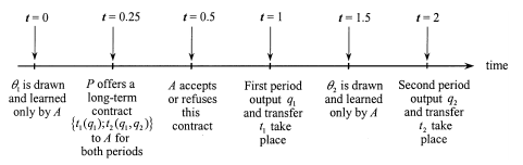
Figure 8.2: Timing with a Twice-Repeated Adverse Selection Problem and Independent Types
Let us also denote the first-period rents by ![]() . At date t = 1, given that the expected continuation rent for period 2 is
. At date t = 1, given that the expected continuation rent for period 2 is ![]()
![]() , the incentive compatibility constraints are written as
, the incentive compatibility constraints are written as

The agent’s intertemporal participation constraints are finally written as

Clearly (8.8) and (8.11) are both binding at the optimum of the principal’s problem.5 Using (8.11), the expected rents for period 2 are written, depending on the first report period, as
![]()
and
![]()
Then, following the logic of section 2.11, the following second period rents satisfy (8.6) and (8.7) without justifying any allocative distortion at date ![]()
![]() :
:

and

Hence, the optimal outputs corresponding to the inefficient draws of types in both periods are such that ![]() , respectively. The agent gets a positive rent only when he is efficient at date t = 1, and his expected intertemporal rent over both periods is
, respectively. The agent gets a positive rent only when he is efficient at date t = 1, and his expected intertemporal rent over both periods is ![]() . In summary, we get proposition 8.2.
. In summary, we get proposition 8.2.
Proposition 8.2: With independent types and a risk-neutral agent, the optimal long-term contract for two periods with full commitment com- bines the optimal static contract written interim for period 1 and the optimal static contract written ex ante for period 2. In particular, the expected rent of the agent only equals the expectation of the agent’s rent when he is efficient in period one and is worth ![]() .
.
Remark: The same result would also be obtained if the risk-neutral agent could leave the relationship in period 2 if he does not get a positive expected rent in this period. In this case, the second period participation constraint
![]()
for all ![]() , must be satisfied. It is then enough to fix
, must be satisfied. It is then enough to fix ![]() and
and ![]() so that the right-hand sides of (8.12) and (8.13) are both equal to zero.
so that the right-hand sides of (8.12) and (8.13) are both equal to zero.
3. Correlated Types and Infinite Risk Aversion
Let us generalize the previous information structure and turn now to the more general case where the agent’s types are imperfectly correlated over time. We denote by ν1 (resp. 1 − ν1) the probability that the first period cost is θ (resp. θ¯). Similarly, we denote the second period probabilities that the agent is efficient (resp. inefficient) by ν2(θ1) (resp. 1 − ν2(θ1)), following a cost realization θ1 in the first period. A positive correlation between costs in both periods is obtained when ![]() .
.
Let us assume that the contract is offered ex ante and that the agent is infinitely risk averse below zero wealth in both periods or, alternatively, that the agent is risk-neutral and protected by limited liability. This imposes that the agent’s payoff in any period must remain positive, whatever his type.
The timing of the game is the same as in figure 8.2. In this framework, a direct revelation mechanism requires that the agent reports the new information in each period he has learned on his current type. Typically, a direct revelation mechanism is a four-uple ![]() for all pairs
for all pairs ![]() belonging to Θ2, where θ1˜ (resp. θ2˜) is the date t = 1 (resp. date t = 2) announcement on his first-period (resp. second-period) type.
belonging to Θ2, where θ1˜ (resp. θ2˜) is the date t = 1 (resp. date t = 2) announcement on his first-period (resp. second-period) type.
The important point to note here is that the first-period report can now be used by the principal to update his beliefs on the agent’s second period type. This report can be viewed as an informative signal that is useful for improving second- period contracting. This idea is quite similar to that seen in section 2.14.1. The difference is that now the signal used by the principal to improve second-period contracting is not exogenously given by nature but comes from the first-period report θ1˜ of the agent on his type θ1. Hence, this signal can be strategically manip- ulated by the agent in the first period in order to improve his second-period rent. This effect will thus affect the way we write intertemporal incentive constraints.
At date t = 2, following a first-period report θ1˜ made by the agent, the prin- cipal will choose outputs ![]() for the efficient type and
for the efficient type and ![]() ) for the inefficient type. The agent will also be proposed second-period rents
) for the inefficient type. The agent will also be proposed second-period rents ![]() . Of course, we have
. Of course, we have ![]() .
.
Because the agent is infinitely risk averse below zero wealth, his ex post par-ticipation constraint in period 2 is written as
![]()
and
![]()
Moreover, inducing information revelation by the agent in period 2 requires to satisfy the following incentive constraints:

Summing those two incentive constraints yields the usual monotonicity con-ditions ![]() .
.
Because of full commitment, the second-period outputs q2(θ1˜) are decided at the time of the offering of the long term contract. Given these outputs, the continuation of the optimal contract for the second period calls for second-period rents that must solve, for any first-period announcement θ1˜, the following problem:

(8.19) and (8.21) are both binding,8 and the principal’s second-period profit, denoted thereafter by ![]() , is written as a function of second- period outputs:
, is written as a function of second- period outputs:

Let us now go back to period 1. Knowing what will be the consequences of his first-period report θ1˜ on the principal’s updated beliefs, the agent with a low first-period cost will truthfully reveal his type whenever the following intertemporal incentive constraint is satisfied:
![]()
where ![]() are the first-period rents. The terms
are the first-period rents. The terms ![]() instead represent the discounted expected infor- mation rents that the agent can get in the second-period continuation of the con- tract if he reports, respectively,
instead represent the discounted expected infor- mation rents that the agent can get in the second-period continuation of the con- tract if he reports, respectively, ![]() to the principal at date t = 1, knowing that the probability that his second-period type is θ is ν2(θ).
to the principal at date t = 1, knowing that the probability that his second-period type is θ is ν2(θ).
Similarly, the agent with a high first-period cost reveals truthfully when
![]()
Summing (8.24) and (8.25) yields the following implementability condition:
![]()
Note that a positive correlation of types across periods implies that ν2(θ¯) < ν2(θ), and thus the implementability condition above is automatically satisfied when ![]() in the first period and
in the first period and ![]() in the second period. As usual, we will not address this condition but instead let the reader check ex post that it is indeed satisfied.
in the second period. As usual, we will not address this condition but instead let the reader check ex post that it is indeed satisfied.
Again, infinite risk aversion below zero wealth requires that the ex post par- ticipation constraints for the first period

are both satisfied.
Taking into account the continuation payoffs ![]() that the principal gets following a first-period announcement θ1˜, the principal’s optimal long-term contract with full commitment is thus the solution to:
that the principal gets following a first-period announcement θ1˜, the principal’s optimal long-term contract with full commitment is thus the solution to:

The two relevant constraints are the incentive constraint (8.24) and the par- ticipation constraint in (8.27). Proposition 8.3 summarizes the dynamics of the optimal long-term contract.
Proposition 8.3: With a positive correlation of types and infinite risk aversion at zero wealth, the optimal long-term contract with full com- mitment entails, for δ small enough:
- Constraints in (8.24) and (8.27) are the only binding constraints for δ small enough.
- The agent always produces the first-best output when he is efficient.
- The agent generally produces below the first-best output when he is inefficient.
In period 1, the inefficient agent produces:
![]()
In period 2, following θ1 = θ¯, the inefficient agent produces:
![]()
In period 2, following θ1 = θ, the inefficient agent produces the first- best output ![]() .
.
- The agent’s expected information rent over both periods is
![]()
To derive proposition 8.3 we have assumed that the first period participation con- straint of the efficient type, i.e., ![]() ,was always strictly satisfied. Indeed, when, (8.24) and (8.27) are both binding, we have
,was always strictly satisfied. Indeed, when, (8.24) and (8.27) are both binding, we have ![]()
![]() is positive as long as the first-period rent
is positive as long as the first-period rent ![]() is larger than the second-period expected rent differential
is larger than the second-period expected rent differential ![]() , which is posi-tive because
, which is posi-tive because ![]() . This condition always holds for small enough δ. Then, for an agent who is efficient in the first period, the second-period expected rent can be recaptured in period 1, and the principal can afford an efficient production level
. This condition always holds for small enough δ. Then, for an agent who is efficient in the first period, the second-period expected rent can be recaptured in period 1, and the principal can afford an efficient production level ![]() for the inefficient type in period 2, following an announcement of θ in period 1. However, for an inefficient agent who has no rent in period 1, this process is not possible. Hence, the principal requires some output distortion for an inefficient type in period 2 following the announcement of θ¯ in period 1.
for the inefficient type in period 2, following an announcement of θ in period 1. However, for an inefficient agent who has no rent in period 1, this process is not possible. Hence, the principal requires some output distortion for an inefficient type in period 2 following the announcement of θ¯ in period 1.
Intuitively, distorting ![]() downward not only helps to reduce the second- period rent of the agent when he is efficient in period 2 following θ1 = θ¯, but it also helps to reduce the cost of the first-period incentive constraint (8.24). There are thus two reasons to distort this output downward, and the corresponding distortion is greater than for the optimal static contract that the principal would offer if his beliefs put a probability ν2(θ¯) on the agent being efficient. On the contrary, reducing
downward not only helps to reduce the second- period rent of the agent when he is efficient in period 2 following θ1 = θ¯, but it also helps to reduce the cost of the first-period incentive constraint (8.24). There are thus two reasons to distort this output downward, and the corresponding distortion is greater than for the optimal static contract that the principal would offer if his beliefs put a probability ν2(θ¯) on the agent being efficient. On the contrary, reducing ![]() helps to reduce the second-period rent of the agent when he is efficient in period 2 following θ1 = θ, but increasing
helps to reduce the second-period rent of the agent when he is efficient in period 2 following θ1 = θ, but increasing ![]() also helps to reduce the cost of the first-period incentive constraint (8.24). These two effects compensate each other exactly so that there is no allocative distortion and
also helps to reduce the cost of the first-period incentive constraint (8.24). These two effects compensate each other exactly so that there is no allocative distortion and ![]() .
.
The main lesson of this section is that the past history of reports plays a role in determining the continuation of the optimal long term contract. Indeed, the principal can use these continuations to relax the cost of the first-period incentive compatibility constraint. In this section, the link between the past history of the agent’s performances and the current production he is asked to produce comes from the intertemporal correlation of types and the informativeness of those past performances on future realizations of the efficiency parameter. We will see in section 8.2.4 how the past history of performances can also be useful to smooth the cost of a risk-averse agent’s incentive compatibility constraint, even when shocks are identically distributed over time.9
Remark 1: Note that the results of proposition 8.3 encompass both the case of independent draws and the case of perfectly correlated draws when the agent is infinitely risk averse below zero wealth in both periods. For independent draws, we have ![]() , and we find that the second-period average marginal surplus with an inefficient type is equal to its first-period value:
, and we find that the second-period average marginal surplus with an inefficient type is equal to its first-period value: ![]()
![]() denotes the expectation operator with respect to θ1˜. In the case of perfectly correlated types, we have instead
denotes the expectation operator with respect to θ1˜. In the case of perfectly correlated types, we have instead ![]() and ν2(θ) = 1. Hence, as in section 8.1.1, the only second-period inefficient output produced with a positive probability is such that
and ν2(θ) = 1. Hence, as in section 8.1.1, the only second-period inefficient output produced with a positive probability is such that ![]() now produced with zero probability.
now produced with zero probability.
Remark 2: It is worth stressing again that the optimal contract found in proposition 8.3 uses the assumption of full commitment. Indeed, the production ![]() has been excessively distorted downwards to induce easier information revelation in period 1 and relax the intertemporal incentive constraint (8.25). When the second period comes, the first-period type has been revealed, and the principal does not have to distort as much the second-period output to induce a less costly revelation of types at this date.
has been excessively distorted downwards to induce easier information revelation in period 1 and relax the intertemporal incentive constraint (8.25). When the second period comes, the first-period type has been revealed, and the principal does not have to distort as much the second-period output to induce a less costly revelation of types at this date.
Baron and Besanko (1984b) derived optimal contracts with types cor- related over time and full commitment of the principal. Laffont and Tirole (1996) provided an application of dynamic contracting models with adverse selection to characterize the optimal regulation of pollution rights. They also gave an interpretation of the optimal mechanisms in terms of mar- kets with options. The case of types independently distributed has also been used in models of infinitely repeated relationships, starting with Townsend (1982), Green (1987), Phelan and Townsend (1991), Green and Oh (1991), Atkeson and Lucas (1992), Thomas and Worrall (1990), and Wang (1995). These authors are interested in deriving the properties of the long run dis- tribution of the agent’s utility and consumption, and sometimes draw some macroeconomic implications from the analysis of these distributions. Gener- ally, the focus of this line of research is on the role of a long-term contract as a substitute to self- or co-insurance. These papers start with the assumption that the agent has a finite (and positive) degree of absolute risk aversion. They also assume that screening in a one-shot relationship is not feasible, because the principal has only one instrument to control the agent, namely the transfers (or the consumption) of the agent in a given period. In a long-term relation- ship, the specification of the continuation payoffs of the contracts is then the second crucial instrument needed to screen the agent. In section 8.2.6 below, we will analyze, for the case of infinitely repeated moral hazard, some of the recursive techniques used in this latter literature to characterize the optimal long-term contract.
4. A Digression on Noncommitment
From the analysis above, it appears that the generalization of incentive theory to a dynamic context is straightforward, provided that the principal has the ability to commit. However, in the case where there is some correlation of types between both periods, the principal could use the information learned in the first period to propose a renegotiation of the initial long-term contract he has initially offered to improve the terms of the rent extraction-efficiency trade-off over the course of the contract. In other words, the optimal long-term contract with full commitment may fail to be renegotiation-proof. In section 2.12 we have already touched on this commitment issue in one-shot relationships, arguing that a simple, indirect mechanism can be a way around this commitment problem and that the possibil- ity for renegotiating the contract comes partly as an artifact of the use of a direct revelation mechanism between the principal and the agent. In an intertemporal context, the commitment problem is much more of a concern. This concern arises because the course of actions leaves open dates for recontracting, and the infor- mation revelation is not an artifact of the modelling but corresponds to physical decisions. It is beyond the scope of this volume to solve for the optimal dynamic renegotiation-proof long-term contract. However, in section 9.4 we provide some preliminary formal analysis of the important trade-off between ex post efficiency and ex ante incentives, which arises when renegotiation is allowed.
Source: Laffont Jean-Jacques, Martimort David (2002), The Theory of Incentives: The Principal-Agent Model, Princeton University Press.