Marginal cost pricing

Marginal cost pricing is the pricing of a product so that it covers the cost of producing one extra unit of the product.

Marginal cost pricing method is frequently used in public services and utilities where the aim is to maximize the economic welfare of the state.

In reality, deficits can arise for a firm with declining average total costs (and consequently falling marginal costs) as prices, if set to equal marginal cost, fail to cover fixed costs.

Also see: average cost pricing, mark-up pricing

Source:
R Rees, Public Enterprise Economics (London, 1984);
P L Joskow, ‘Contributions of the Theory of Marginal Cost Pricing’, Bell Journal of Economics, 7, 1 (Spring, 1976), 197-206

Short run marginal cost

Short Run Marginal Cost

Short run marginal cost is the change in total cost when an additional output is produced in the short run. Based on the Short Run Marginal Cost graph on the right side of the page, SMC forms a U-shape in a graph where the x-axis plays the quantity and the y-axis costs. Cost curves are all U-shaped due to the law of variable proportions. This includes marginal costs together with average variable costs and average total costs.^[4]

On the short run, firms often have a fixed number of assets (eg. equipment, machinery). The firm owner can choose to increase or decrease productivity with the current amount of assets he has. When choosing to increase or decrease productivity, there is a single point where the unit cost reaches the minimum level (lowest point of marginal cost). At this point, the short-run average total cost is utilized with the optimal combination of both variable and fixed cost.^[4]

Long run marginal cost

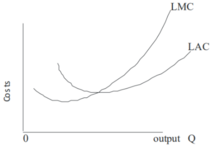
Long Run Marginal Cost

Fixed factors of production in the long run does not exist, therefore, we will not be using the fixed and variable factors. The concept is fairly similar to short run marginal cost minus the application of fixed cost. As seen in the graph, there are fixed costs.^[4]

Cost functions and relationship to average cost

In the simplest case, the total cost function and its derivative are expressed as follows, where Q represents the production quantity, VC represents variable costs, FC represents fixed costs and TC represents total costs.

Fixed costs represent the costs that do not change as the production quantity changes. Fixed costs are costs incurred by things like rent, building space, machines, etc. Variable costs change as the production quantity changes, and are often associated with labor or materials. The derivative of fixed cost is zero, and this term drops out of the marginal cost equation: that is, marginal cost does not depend on fixed costs. This can be compared with average total cost (ATC), which is the total cost (including fixed costs, denoted C₀) divided by the number of units produced:

{\displaystyle ATC={\frac {C_{0}+\Delta C}{Q}}.}

For discrete calculation without calculus, marginal cost equals the change in total (or variable) cost that comes with each additional unit produced. Since fixed cost does not change in the short run, it has no effect on marginal cost.

For instance, suppose the total cost of making 1 shoe is $30 and the total cost of making 2 shoes is $40. The marginal cost of producing shoes decreases from $30 to $10 with the production of the second shoe ($40 – $30 = $10).

Marginal cost is not the cost of producing the “next” or “last” unit.^[5] The cost of the last unit is the same as the cost of the first unit and every other unit. In the short run, increasing production requires using more of the variable input — conventionally assumed to be labor. Adding more labor to a fixed capital stock reduces the marginal product of labor because of the diminishing marginal returns. This reduction in productivity is not limited to the additional labor needed to produce the marginal unit – the productivity of every unit of labor is reduced. Thus the cost of producing the marginal unit of output has two components: the cost associated with producing the marginal unit and the increase in average costs for all units produced due to the “damage” to the entire productive process. The first component is the per-unit or average cost. The second component is the small increase in cost due to the law of diminishing marginal returns which increases the costs of all units sold.

Marginal costs can also be expressed as the cost per unit of labor divided by the marginal product of labor.^[6] Denoting variable cost as VC, the constant wage rate as w, and labor usage as L, we have

{\displaystyle MC={\frac {\Delta VC}{\Delta Q}}}

{\displaystyle \Delta VC={w\Delta L}}

{\displaystyle MC={\frac {w\Delta L}{\Delta Q}}={\frac {w}{MPL}}.}

Here MPL is the ratio of increase in the quantity produced per unit increase in labour: i.e. ΔQ/ΔL, the marginal product of labor. The last equality holds because {\displaystyle {\frac {\Delta L}{\Delta Q}}} is the change in quantity of labor that brings about a one-unit change in output.^[7] Since the wage rate is assumed constant, marginal cost and marginal product of labor have an inverse relationship—if the marginal product of labor is decreasing (or, increasing), then marginal cost is increasing (decreasing), and AVC = VC/Q=wL/Q = w/(Q/L) = w/AP_L