It is often the case that the agent does not exert a single-dimensional effort, par- ticularly when he is involved in many related activities associated with the same job. Such examples abound, as we will see in section 5.2.5 below. When the agent simultaneously performs several tasks for the principal, new issues arise: How does the technological interaction among those tasks affect incentives? What sort of optimal incentive contracts should be provided to the agent? How do incentive considerations affect the optimal mix of efforts along each dimension of the agent’s performance?
1. Technology
To answer the above questions, we now extend the simple model of chapter 4 and let the agent perform two tasks for the principal with respective efforts e1 and e2. For simplicity, we first assume that those two tasks are completely symmetric and have the same stochastic returns Si = S¯ or S, for i = 1, 2. Those returns are independently distributed with respective probabilities π(e1) and π(e2). Since there are basically only three possible outcomes, yielding 2S¯,S¯ + S, and 2S to the principal, a contract is in fact a triplet of corresponding payments ![]() is given in case of success on both tasks, tˆ is given in case of success on only one task and t is given when none of the tasks has been successful.
is given in case of success on both tasks, tˆ is given in case of success on only one task and t is given when none of the tasks has been successful.
Again, we normalize each effort to belong to {0, 1}. Note that the model has, by symmetry, three possible levels of aggregate effort. The agent can exert a high effort on both tasks, on only one task, or on no task at all. The reader will recognize that the multitask agency model should thus inherit many of the difficulties discussed in section 5.1. However, the multitask problem also has more structure thanks to the technological assumption generally made on these tasks. We will denote by ψ2, ψ1, and ψ0 = 0 the agent’s disutilities of effort when he exerts, respectively, two high-effort levels, only one, or none. Of course, we have ψ2> ψ1 > 0. Moreover, we say that the two tasks are substitutes when ψ2 > 2ψ1, and complements when instead ψ2 < 2ψ1. When tasks are substitutes, it is harder to accomplish the second task at the margin when the first one is already performed. The reverse holds when the two tasks are complements.
2. The Simple Case of Limited Liability and Substitutability of Tasks
In this section we begin by analyzing a simple example with a risk-neutral agent protected by limited liability.
First-Best Outcome
Let us first assume that the principal performs the tasks himself, or alternatively that he uses a risk-neutral agent to do so and that effort is observable.
Because the performances on each task are independent variables, the prin- cipal’s net benefit of choosing to let the agent exert a positive effort on both tasks is ![]() . Note also that C2FB = ψ2 is the first-best cost of implementing both efforts in this case of risk neutrality.
. Note also that C2FB = ψ2 is the first-best cost of implementing both efforts in this case of risk neutrality.
If he chooses to let the agent exert only one positive level of effort, the prin- cipal instead gets ![]() . The first-best cost of implementing only one effort is then C1FB = ψ1.
. The first-best cost of implementing only one effort is then C1FB = ψ1.
Finally, if he chooses to let the agent exert no effort at all, the principal gets ![]()
Hence, exerting both efforts is preferred to any other allocation when V2FB ≥ max(V2FB, V0FB), or to put it differently, when
![]()
When the two tasks are substitutes, we have ![]() . The more stringent constraint on the right-hand side of (5.31) is obtained when the principal lets the agent exert one positive level of effort.14 Figure 5.2 summarizes the first-best choices of effort made by the principal as a function of the incremental benefit ΔπΔS associated with each task.
. The more stringent constraint on the right-hand side of (5.31) is obtained when the principal lets the agent exert one positive level of effort.14 Figure 5.2 summarizes the first-best choices of effort made by the principal as a function of the incremental benefit ΔπΔS associated with each task.
When tasks are substitutes a whole range of intermediate values of ΔπΔS exist, which are simultaneously large enough to justify a positive effort on one task and small enough to prevent the principal from willing to let the agent exert both efforts.
Moral Hazard
Let us now turn to the case where efforts are nonobservable and the risk-neutral agent is protected by limited liability.

Figure 5.2: First-Best Levels of Effort with Substitutes
Suppose first that the principal wants to induce a high effort on both tasks. We leave it to the reader to check that the best way to do so is for the principal to reward the agent only when q˜1 = q˜2 = q¯, i.e., when both tasks are successful. Differently stated, we have ![]() .
.
The local incentive constraint that prevents the agent from exerting only one effort is written as
![]()
The global incentive constraint that prevents the agent from exerting no effort at all is instead written as
![]()
Both incentive constraints (5.32) and (5.33) can finally be summarized as
![]()
The principal’s problem (P) is thus written as:

The latter constraint is obviously binding at the optimum of (P). The second- best cost of implementing both efforts is thus ![]() . For the principal, the net benefits from inducing a positive effort on both activities is written as
. For the principal, the net benefits from inducing a positive effort on both activities is written as
![]()
If the principal chooses to induce only one effort, e.g., on task 1, he instead offers a transfer ![]() each time that q˜1 = q¯ and zero otherwise, just as in chapter 4. The second-best cost of implementing effort on a single task is thus
each time that q˜1 = q¯ and zero otherwise, just as in chapter 4. The second-best cost of implementing effort on a single task is thus ![]() .
.
The second-best net benefit for the principal of inducing this single dimension of effort is
![]()
Again, there are three possible sets of parameters, characterizing different zones for which the principal wants to induce either zero, one, or two efforts.
It is easy to check that the principal now chooses to exert zero effort more often than under complete information, because
![]()
Let us turn to the determination of whether or not the principal induces two positive efforts under moral hazard less often than under complete information.
We isolate two cases. First, when ![]() , one can check that the local incentive constraint is the more constraining one for a principal willing to induce both efforts from the agent. This means that
, one can check that the local incentive constraint is the more constraining one for a principal willing to induce both efforts from the agent. This means that ![]() . Then, the inequality
. Then, the inequality ![]() implies that
implies that
![]()
This inequality means that the principal induces those two efforts less often than under complete information (figure 5.3).
The intuition behind this result is the following. Under moral hazard, the cost of implementing either two efforts or one effort is greater than under complete information. Because of the technological substitutability between tasks, what mat- ters for evaluating whether both tasks should be incentivized less often than under complete information is how the second-best incremental cost C2SB − C1SB can be compared to the first-best incremental cost CFB − CFB. When the local incentive

constraint is binding it is harder to incentivize effort on a second task when a positive effort is already implemented on the first one. The second-best cost of inducing effort increases more quickly than the first-best cost as one goes from one task to two tasks.
Remark: Note that π0 < π1 implies that the condition ![]() is more stringent than the condition for task substitutability, namely ψ2 > 2ψ1. For the second-best cost of implementation to satisfy (5.38), it must be true that efforts are in fact strong substitutes. It is then much harder to accomplish the second task at the margin when the first one is already done.
is more stringent than the condition for task substitutability, namely ψ2 > 2ψ1. For the second-best cost of implementation to satisfy (5.38), it must be true that efforts are in fact strong substitutes. It is then much harder to accomplish the second task at the margin when the first one is already done.
Let us now turn to the case where ![]() . For such a weak substi-tutability, the global incentive constraint is now the more constraining one for a principal willing to induce both efforts from the agent. The transfer received by the agent is thus
. For such a weak substi-tutability, the global incentive constraint is now the more constraining one for a principal willing to induce both efforts from the agent. The transfer received by the agent is thus ![]() implies that we also have
implies that we also have
![]()
The principal now prefers to induce both efforts rather than only one more often than under complete information. The second-best cost of inducing effort increases less quickly than the first-best cost as one goes from one task to two tasks. Intu- itively, incentives create a complementarity between tasks which goes counter to the technological diseconomies of scope.
We summarize these findings in proposition 5.4.
Proposition 5.4: Under moral hazard and limited liability, the degree of diseconomies of scope between substitute tasks increases or decreases depending on whether local or global incentive constraints are binding in the principal’s problem.
The Case of Complements
Let us briefly discuss the case where the two tasks are complements. Figure 5.4 describes the values of benefit for which the principal wants to induce both efforts.
Under moral hazard, the global incentive constraint is now always binding for a principal willing to induce both efforts. Indeed, the inequality ![]() always holds when ψ2 < 2 ψ1 . Hence, we have also
always holds when ψ2 < 2 ψ1 . Hence, we have also ![]() . The principal
. The principal![]() now finds it harder to induce both efforts than under complete information, as can be seen in figure 5.5.
now finds it harder to induce both efforts than under complete information, as can be seen in figure 5.5.

Figure 5.4: First-Best Levels of Effort with Complements
 Figure 5.5: Second-Best Levels of Effort with Complements
Hence, the principal induces a pair of high efforts under moral hazard less often than under complete information. Intuitively, the case of complementarity is very much like the case of a single activity analyzed in chapter 4.
3. The Optimal Contract with a Risk-Averse Agent
In this section and the following one we assume that the agent is strictly risk- averse. Because of the symmetry between tasks, there is again no loss of generality in assuming that the principal offers a contract ![]() where t¯ is given in case of success on both tasks, tˆ is given when only one task is successful, and t is given when no task succeeds.
where t¯ is given in case of success on both tasks, tˆ is given when only one task is successful, and t is given when no task succeeds.
Let us now describe the set of incentive feasible contracts that induce effort on both dimensions of the agent’s activity. As usual, it is useful to express these constraints with the agent’s utility levels in each state of nature as the new variables.
Let us thus define ![]() . We have to consider the possibility that the agent could shirk, not only on one dimension of effort but also on both dimensions. The first incentive constraint is a local incentive constraint which is written as
. We have to consider the possibility that the agent could shirk, not only on one dimension of effort but also on both dimensions. The first incentive constraint is a local incentive constraint which is written as

The second incentive constraint is instead a global incentive constraint and is written as

Finally, the agent’s participation constraint is
![]()
If he wants to induce both efforts, the principal’s problem can be stated as:

Structure of the Optimal Contract
A priori, the solution to problem (P) may entail that either one or two incentive constraints is binding. Moreover, when there is only one such binding constraint it might be either the local or the global incentive constraint. We derive the full-fledged analysis when the inverse utility function h = u−1 is quadratic, i.e., ![]() for some r > 0 and u ≥ − 1/r , in appendix 5.1. The next proposition ummarizes our findings.
for some r > 0 and u ≥ − 1/r , in appendix 5.1. The next proposition ummarizes our findings.
Proposition 5.5: In the multitask incentive problem (P) with h(u) = u + ru2/2 (r>0), the optimal contract that induces effort on both tasks is such that the participation constraint (5.42) is always binding. Moreover, the binding incentive constraints are:
- The local incentive constraint (5.40) in the case of substitute tasks, such that ψ2 > 2ψ1.
- Both the local and the global incentive constraints (5.40) and (5.41) in the case of weak complement tasks, such that

- The global incentive constraint (5.41) in the case of strong complement tasks, such that
The incentive problem in a multitask environment with risk aversion has an intuitive structure that is somewhat similar to the one obtained in section 5.2.2. When efforts are substitutes, the principal finds it harder to provide incentives for both tasks simultaneously than it was for only one task. Indeed, the agent is more willing to reduce his effort on task 1 if he already exerts a high effort on task 2. The local incentive constraint is thus binding. On the contrary, with a strong complementarity between tasks, inducing the agent to exert a positive effort on both tasks simultaneously rather than on none becomes the most difficult constraint for the principal. The global incentive constraint is now binding. For intermediary cases, i.e., with weak complements, the situation is less clear. All incentive constraints, both local and global ones, are then binding.
Remark: The reader will have recognized the strong similarity between the structure of the optimal contract in the moral hazard multitask problem and the structure of the optimal contract in the multidimensional adverse selection problem that was discussed in section 3.2. In both cases, it may happen that either local or global incentive constraints bind. A strong complementarity of efforts plays almost the same role as a very strong correlation in the agent’s types under adverse selection. It makes it more likely that the global incentive constraint binds.
Optimal Effort
Let us turn now to the characterization of the optimal effort chosen by the principal in this second-best environment. To better understand these choices it is useful to start with the simple case where tasks are technologically unrelated, i.e., ψ2 = 2ψ1.
Suppose that the principal wants to induce effort on only one task. Under complete information, the expected incremental benefit of doing so, ΔπΔS, should exceed the first-best cost C1FB of implementing this effort:
![]()
With two tasks, and still under complete information, the principal prefers to induce effort on both tasks rather than on only one when the incremental expected benefit from implementing one extra unit of effort, which is again ΔπΔS, exceeds the increase in the cost of doing so, i.e., C2FB − C1FB, where C2FB = h(2ψ1) = ![]() is the first-best cost of implementing two efforts. This leads to the condition
is the first-best cost of implementing two efforts. This leads to the condition
![]()
It is easy to check that the right-hand side of (5.44) is greater than the right- hand side of (5.43), because C2FB > 2C1FB as soon as r > 0. When ΔπΔS belongs to [C1FB, C2FB − C1FB] only one effort is induced. Note for further reference that this interval has a positive length C2FB − 2C1FB.
Moreover, the inequality C2FB − C1FB > C1FB means that it is less often valuable for the principal to induce both efforts rather than inducing one effort when effort is verifiable. The latter inequality also means that the first-best cost of implement- ing efforts exhibits some diseconomies of scope. Adding up tasks makes it more costly to induce effort from the agent, even if those tasks are technologically unre- lated and contracting takes place under complete information. The point here is that inducing the agent to exert more tasks requires increasing the certainty equivalent income necessary to satisfy his participation constraint. Adding more tasks therefore changes the cost borne by the principal for implementing an extra level of effort. Now that the agent has a decreasing marginal utility of consump- tion, multiplying the level of effort by two requires multiplying the transfer needed to ensure the agent’s participation by more than two. For that reason, the disec- onomies of scope isolated above can be viewed as pure participation diseconomies of scope.
Now, still with unrelated tasks, let us move to the case of moral hazard. Under moral hazard, we already know from section 4.4 that, with the specification made on the agent’s utility function, the second-best cost of implementing a single effort is written as

The principal now prefers to induce one effort rather than none when
![]()
i.e., less often than under complete information.
In appendix 5.2, we also compute C2SB to be the second-best cost of imple-menting a positive effort on both tasks. For unrelated tasks this cost writes as

This cost again has an intuitive meaning. Since tasks are technologically unrelated, providing incentives on one of those tasks does not affect the cost of incentives on the other. Just as in chapter 4, the principal must incur an agency cost ![]() per task on top of the complete information cost C2FB that is needed to ensure the agent’s participation.
per task on top of the complete information cost C2FB that is needed to ensure the agent’s participation.

Figure 5.6: First-Best and Second-Best Efforts with Unrelated Tasks
Given this agency cost, the principal prefers to induce two positive efforts rather than only one when
![]()
(5.48) is more stringent than (5.46), because C2SB > 2C1SB.
When ΔπΔS belongs to [C2SB, C2SB − C1SB], only one effort is induced under moral hazard and this interval has length C2SB − 2C1SB. In fact, one can easily observe that the second-best rules (5.48) and (5.46) are respectively “translated” from the first-best rules (5.44) and (5.43) by adding the same term ![]() , which is precisely the extra cost paid by the principal to induce a positive effort on a single dimension of the agent’s activities when there is moral hazard.
, which is precisely the extra cost paid by the principal to induce a positive effort on a single dimension of the agent’s activities when there is moral hazard.
We conclude from this analysis that, with technologically unrelated tasks, agency problems do not reduce the set of parameters over which the principal induces only one effort from the agent, because C2SB − 2C1SB = C2FB − 2C1FB. This can be seen in figure 5.6.
Let us now turn to the more interesting case where efforts are substitutes, i.e.,ψ2 > 2ψ1. On top of the participation diseconomies of scope already seen above, our analysis will highlight the existence of incentives diseconomies of scope. To see their origins, we proceed as before and first analyze the complete information decision rule. The principal still prefers to induce one effort rather than none when (5.43) holds. However, the principal prefers now to induce two efforts rather than only one when
![]()
where ![]()
Again, we can check that the right-hand side of (5.49) is greater than the right-hand side of (5.43) since
![]()
where the first inequality uses the facts that h(·) is increasing and that ψ2 > 2ψ1 and the second inequality uses the convexity of h(·).
Moving now to the case of moral hazard, the principal still prefers to induce one effort rather than none when (5.46) holds. Moreover, the second-best cost of inducing two efforts is now17

Again, this expression has an intuitive meaning. In order to induce the agent to exert two efforts that are substitutes, the principal must consider the more con- straining local incentive constraint, which prevents the agent from exerting effort on only one dimension of his activities. For each of those two local incentive constraints,18 the incentive cost that should be added to the first-best cost of imple-menting both efforts is ![]() , where ψ2 – ψ1 is the incremental disutility of effort when moving from one effort to two efforts.
, where ψ2 – ψ1 is the incremental disutility of effort when moving from one effort to two efforts.
Hence, the principal prefers to induce both efforts rather than only one when
![]()
In a second-best environment, both efforts are incentivized less often than only one. Indeed, the second-best decision rule to induce both efforts (5.52) is more stringent than the second-best decision rule (5.46) to induce only one, since

We notice that again there are some diseconomies of scope in implementing both efforts. However, those diseconomies of scope now have a double origin. First, there are the participation diseconomies of scope that ensure that (5.50) holds under complete information. Second, and contrary to the case of technologically unrelated tasks, incentives diseconomies of scope now appear, since

if and only if ψ2 > 2ψ1.
Moving from the first-best world to the case of moral hazard it becomes even harder to induce effort on both tasks rather than on only one because of these incentives diseconomies of scope. Figure 5.7 graphically shows the impact of these new agency diseconomies of scope on the optimal decision rule followed by the principal.
We also summarize our findings in proposition 5.6.
Proposition 5.6: When tasks are substitutes and entail moral hazard, the principal must face some new incentives diseconomies of scope that reduce the set of parameters such that inducing both efforts is second-best optimal.
This proposition highlights the new difficulty faced by the principal when incentivizing the agent on two tasks under moral hazard. Incentives diseconomies of scope imply that the principal will choose to induce effort on only one task more often than under complete information. Task focus may be a response to these agency diseconomies of scope.
Remark: The case of complements could be treated similarly. It would highlight that incentives economies of scope exist when an agent per- forms two tasks that are complements.

Figure 5.7: First-Best and Second-Best Efforts with Substitute Tasks
4. Asymmetric Tasks
The analysis that we have performed in section 5.2.3 was simplified by our assump- tion of symmetry between the two tasks. In a real world contracting environment, those tasks are likely to differ along several dimensions, such as the noises in the agent’s performances, the expected benefits of those tasks, or the sensitivity of the agent’s performance on his effort. The typical example along these lines is that of a university professor who must devote effort to both research and teaching. Those two tasks are substitutes; giving more time to teaching reduces the time spent on research. Moreover, the performances on each of those tasks cannot be measured with the same accuracy. Research records may be viewed as precise measures of the performance along this dimension of the professor’s activity. Teaching quality is harder to assess.
To model such settings, we now generalize the multitask framework to the case of asymmetric tasks, which we still index with a superscript i in {1, 2}. Task i yields a benefit S¯i to the risk-neutral principal with probability ![]() and a benefit Si with probability 1 − πki when the agent exerts effort eki on task i.
and a benefit Si with probability 1 − πki when the agent exerts effort eki on task i.
Effort eki still belongs to {0, 1}, and we assume the same disutilities of effort as in the symmetric case. Benefits and probabilities distributions may now differ across tasks.
A contract is now a four-uple ![]() where tˆ1 is offered when the outcome is
where tˆ1 is offered when the outcome is ![]() and tˆ2 is offered when
and tˆ2 is offered when ![]() is realized. We must allow for the possibility that tˆ1 is possibly different from tˆ2, contrary to our previous assumption in section 5.2.3. Indeed, to take advantage of the asymmetry between tasks, the principal may want to distinguish these two payments.
is realized. We must allow for the possibility that tˆ1 is possibly different from tˆ2, contrary to our previous assumption in section 5.2.3. Indeed, to take advantage of the asymmetry between tasks, the principal may want to distinguish these two payments.
Let us again use our usual change of variables so that transfers are replaced by utility levels in each state of nature: ![]() , and u = u(t). An incentive feasible contract inducing a positive effort on both tasks must satisfy two local incentive constraints,
, and u = u(t). An incentive feasible contract inducing a positive effort on both tasks must satisfy two local incentive constraints,

and a global incentive constraint,

Finally, a contract must also satisfy the usual participation constraint,
![]()
The principal’s problem is thus written as

Again, to obtain an explicit solution to (P) we specify a quadratic expression for the inverse utility function so that ![]() for some r > 0 and
for some r > 0 and ![]() .
.
The intuition built in section 5.2.3 suggests that local incentive constraints are the most difficult ones to satisfy in the case where tasks are substitutes, i.e., when ψ2 > 2ψ1. This is indeed the case as it is confirmed in the next proposition, which generalizes proposition 5.5 to the case of asymmetric tasks.
Proposition 5.7: When tasks are substitutes, the solution to fP g is such that the local incentive constraints (5.55) and (5.56) and the participation constraint (5.58) are all binding. The global incentive constraint (5.57) is always slack.
Using the second-best values of ![]() that we derive in appendix 5.3, we can compute the second-best cost of implementing two positive levels of effort C2SB. After easy computations, we find that
that we derive in appendix 5.3, we can compute the second-best cost of implementing two positive levels of effort C2SB. After easy computations, we find that

This second-best cost can be given an intuitive interpretation. Under com-plete information, ensuring the agent’s participation costs ![]() to the principal. This is the first term of the right-hand side of (5.59). Under moral haz- ard and with substitute tasks, each of the tasks i can be incentivized by giving a bonus in utility terms
to the principal. This is the first term of the right-hand side of (5.59). Under moral haz- ard and with substitute tasks, each of the tasks i can be incentivized by giving a bonus in utility terms ![]() , with probability π1i, and imposing a punishment
, with probability π1i, and imposing a punishment ![]() with probability 1- π1i. Success and failure on each task being independent events, the incentive costs of inducing those two independent risks in the agent’s payoff just add up. These costs represent the second bracketed term on (5.59). The above expression of C2SB will be used throughout the next subsection.
with probability 1- π1i. Success and failure on each task being independent events, the incentive costs of inducing those two independent risks in the agent’s payoff just add up. These costs represent the second bracketed term on (5.59). The above expression of C2SB will be used throughout the next subsection.
5. Applications of the Multitask Framework
Aggregate Measures of Performances
Let us suppose that ![]() . In this case, the principal, by simply observ- ing the aggregate benefit of his relationship with the agent, cannot distinguish the successful task from the unsuccessful one. The only contracts that can be written are conditional on the agent’s aggregate performance. They are thus of the form
. In this case, the principal, by simply observ- ing the aggregate benefit of his relationship with the agent, cannot distinguish the successful task from the unsuccessful one. The only contracts that can be written are conditional on the agent’s aggregate performance. They are thus of the form ![]() . With respect to the framework of section 5.2.4, everything happens as if a new constraint
. With respect to the framework of section 5.2.4, everything happens as if a new constraint ![]() was added. This restriction in the space of available contracts is akin to an incomplete contract assumption. To show the consequences of such an incompleteness, it is useful to use the expressions for
was added. This restriction in the space of available contracts is akin to an incomplete contract assumption. To show the consequences of such an incompleteness, it is useful to use the expressions for ![]() found in appendix 5.3 to compute the difference of payoffs
found in appendix 5.3 to compute the difference of payoffs ![]() Given this value, the only case where the measure of aggregate performance does as well as the measure of individual performances on both tasks is when Δπ1 = Δπ2, i.e., in the case of symmetric tasks analyzed in section 5.2.3. Otherwise, there is a welfare loss incurred by the principal from not being able to distinguish between the two intermediate states of nature.
Given this value, the only case where the measure of aggregate performance does as well as the measure of individual performances on both tasks is when Δπ1 = Δπ2, i.e., in the case of symmetric tasks analyzed in section 5.2.3. Otherwise, there is a welfare loss incurred by the principal from not being able to distinguish between the two intermediate states of nature.
Let us assume now that Δπ1 < Δπ2. This condition means that task 1 is harder to incentivize than task 2, because an increase of effort has less impact on performances. In this case, ![]() should thus be greater than
should thus be greater than ![]() if the benefits of each task were observable. With only an aggregate measure of performance, the principal is forced to set uˆ1 = uˆ2. Then it becomes more difficult to provide incentives on task 1, which is the more costly task from the incentive point of view, and easier to give incentives on task 2, which is the least costly. Consequently, there may be a misallocation of the agent’s efforts, because he prefers to shift his effort towards task 2. Even if task 1 is as valuable as task 2 for the principal, the latter will find it less often optimal to incentivize this first task.
if the benefits of each task were observable. With only an aggregate measure of performance, the principal is forced to set uˆ1 = uˆ2. Then it becomes more difficult to provide incentives on task 1, which is the more costly task from the incentive point of view, and easier to give incentives on task 2, which is the least costly. Consequently, there may be a misallocation of the agent’s efforts, because he prefers to shift his effort towards task 2. Even if task 1 is as valuable as task 2 for the principal, the latter will find it less often optimal to incentivize this first task.
A simple example illustrates this point. Consider a retailer who must allocate his efforts between improving cost and raising demand for the product he sells on behalf of a manufacturer. If the only observable aggregate is profit, the optimal retail contract is a sharing rule that nevertheless might induce the manager to exert effort only on one task, e.g., the one that consists of enhancing demand, if the latter task is easier to incentivize for the principal.
More or Less Informative Performances
Let us thus assume that the principal can still observe the whole vector of perfor- mances ![]() and offers a fully contingent contract
and offers a fully contingent contract ![]() . We now turn to the rather difficult question of finding the second-best choice of efforts that the principal would like to implement when tasks are asymmetric.
. We now turn to the rather difficult question of finding the second-best choice of efforts that the principal would like to implement when tasks are asymmetric.
We have already derived the second-best cost C2SB of implementing two posi- tive efforts in section 5.2.4. Had the principal chosen to implement a positive effort on task 1 only, the second-best cost of implementing this effort would instead be
![]()
Similarly, the second-best cost of implementing a positive effort on task 2 is written as
![]()
Let us denote the benefits obtained by the principal on each activity when he induces a high level of effort by B1 = Δπ1ΔS1 and B2 = Δπ2ΔS2. The principal prefers to induce e1 = e2 = 1, rather than e1 = e2 = 0, when B1 + B2 − CSB ≥ 0. The principal also prefers to induce e1 = e2 = 1 rather than e1 = 1 and e2 = 0 when B1 + B2 − C2SB ≥ B1 − C1SB. Similarly, e1 = e2 = 1 is preferred to e1 = 0 and e2 = 1 when B1 + B2 − CSB ≥ B2 − C2SB.
Proceeding similarly, we could determine the set of values of the parameters where inducing the pairs of efforts (e1 = 1, e2 = 0) and (e1 = 0, e2 = 1) are respectively optimal. Figure 5.8a, b offers a complete characterization of all these areas of dominance where it has been taken into account that some diseconomies of scope exist in implementing a high effort on both tasks (i.e., C2SB > C1SB + C2SB) when those tasks are substitutes.
In these figures all pairs of parameters (B1, B2) lying on the northeast quadrant of point B justify the implementation of two positive efforts. On the southwest quadrant of point A, no effort is implemented. On the southeast (resp. northwest) of the line joining A and B, only task 1 (resp. task 2) is incentivized.
When the performance on task 2 becomes more noisy, the variance of output q˜2, which is ![]() , increases to
, increases to ![]() . Comparing (5.59) and (5.61), we observe that the cost C2SB increases more quickly than C2SB with this variance. This effect increases the area of parameters (B1, B2) where the principal wants to induce e1 = 1 and e2 = 0, since point A is shifted to Aˆ point B to Bˆ, as can be seen in figure 5.7.
. Comparing (5.59) and (5.61), we observe that the cost C2SB increases more quickly than C2SB with this variance. This effect increases the area of parameters (B1, B2) where the principal wants to induce e1 = 1 and e2 = 0, since point A is shifted to Aˆ point B to Bˆ, as can be seen in figure 5.7.
The intuition behind this phenomenon is clear. When the performance on task 2 becomes a more noisy signal of the corresponding effort, inducing effort along this dimension becomes harder for the principal. By rewarding only the more informative task 1, the principal reduces the agent’s incentives to substitute effort e2 for effort e1. This relaxes the incentive problem on task 1, making it easier to induce effort on this task. More often the principal chooses to have the agent exert effort only on task 1. Finally, the agent receives higher powered incentives only for the less noisy task, the one that is the most informative on his effort. This can be interpreted as saying that the principal prefers that the agent focuses his attention on the more informative activity.21
The Interlinking of Agrarian Contracts
In various contracting environments a principal is not involved in a single trans- action with the agent but requires from the latter a bundle of different services or activities. This phenomenon, called the interlinking of contracts, is pervasive in agrarian economies where landlords sometimes offer consumption services, finance, and various inputs to their tenants. This bundling of different contracting
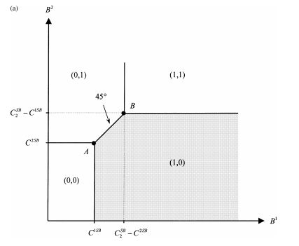

Figure 5.8: (a) Optimal Effort Levels, (b) Optimal Effort Levels when Performance on Task 2 Is More Noisy
activities also occurs in more developed economies when input suppliers also offer lines of credit to their customers.
This phenomenon can be easily modelled within a multitask agency frame- work. To this end, let us consider a relationship between a risk-neutral landlord and a risk-averse tenant similar to that described in section 4.8.2. The landlord and the tenant want to share the production of an agricultural product (the price of which is normalized to one for simplicity). However, and this is the novelty of the multitask framework, the tenant can also make an investment I˜ that, together with his effort, affects the stochastic production process. The probability that q¯ is realized now becomes π(e, I˜) where effort e belongs to {0, 1}. We will also assume that ![]() i.e., a greater investment improves the probability that a high output realizes . For simplicity, we will assume that I˜ can only take two values, respectively 0 and I > 0. Denoting the interest rate by R, the cost incurred by the agent, when investing I, is thus (1 + R)I. If I˜ is not observed by the landlord, the framework is akin to a multitask agency model where the principal would like to control not only the agent’s choice of effort e but also his investment I˜.
i.e., a greater investment improves the probability that a high output realizes . For simplicity, we will assume that I˜ can only take two values, respectively 0 and I > 0. Denoting the interest rate by R, the cost incurred by the agent, when investing I, is thus (1 + R)I. If I˜ is not observed by the landlord, the framework is akin to a multitask agency model where the principal would like to control not only the agent’s choice of effort e but also his investment I˜.
As a benchmark, let us suppose that the investment I is observable and veri- fiable at a cost C by the landlord. If the principal wants to make a positive invest- ment, the incentive feasible contract inducing effort must satisfy the following simple incentive constraint:
Similarly, the following participation constraint must be satisfied:
![]()
The optimal incentive feasible contract inducing effort is thus a solution to the following problem:
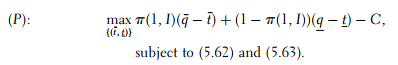
Thereafter we will denote the solution to this problem by t¯v and tv.
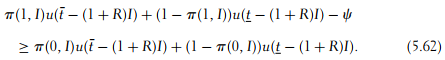
Let us now assume that the investment is nonobservable by the landlord. The choice of the investment level cannot be included in the contract. An incentive feasible contract must now induce the choice of a positive investment if the prin- cipal still finds this investment valuable. Two new incentive constraints must be added to describe the set of incentive feasible contracts. First, the following constraint prevents an agent from simultaneously reducing his effort and his investment:
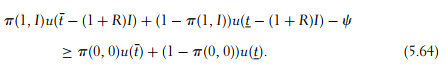
Second, we must take into account the incentive constraint inducing invest-ment when the agent already exerts an effort:
To simplify the analysis of the possible binding constraints, let us also assume that
![]()
This assumption ensures that the investment has more impact on the prob-ability that q¯ is realized when the agent already exerts a positive effort. There is thus a complementarity between effort and investment.
In this case, any contract-inducing effort at minimal cost when the investment is performed will not induce this effort when no such investment is made. Indeed, to check this assertion, note that
![]()
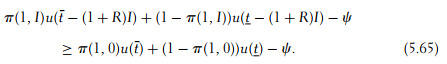
The first inequality uses t¯ > t, and the fact that u(·) is concave. The equality uses the fact that (5.62) is binding if the effort is induced at minimal cost. Finally, the second inequality uses the assumption (5.66). Therefore, (5.64) is more stringent than (5.65). (5.64) may be the more constraining of the incentive constraints when both investment and effort are nonobservable. In this case, the contract offered when I˜ is contractible, namely ![]() , may no longer be optimal. When I˜ is nonobservable, a simultaneous shirking deviation along both the effort and the investment dimensions may occur.
, may no longer be optimal. When I˜ is nonobservable, a simultaneous shirking deviation along both the effort and the investment dimensions may occur.
The benefit of controlling the agent’s investment comes from the reduction in the agency cost. Of course, this benefit should be traded off against the possible fixed cost that the principal would incur if he wanted to establish the monitor- ing system that would make I directly controllable. The interlinking of contracts may thus appear as an institutional response to the technological complementarity between effort and investment in a world where verifying investment is not too costly.
Braverman and Stiglitz (1982) analyzed a model of tenancy-cum- credit contracts, and they show that the landlord may encourage the tenant to get indebted to him when, by altering the terms of the loan contract, he induces the landlord to work harder. Bardhan (1991) reviewed the other justifications for interlinking transactions. In particular, he argued that the interlinking of contracts may help, in nonmonetized economies, by reducing enforcement costs.
Vertical Integration and Incentives
Sometimes it may be hard to contract on the return for some of the agent’s activi- ties. A retailer’s building up of a good reputation or goodwill and the maintenance of a productive asset are examples of activities that are hard or even impossible to measure. Even though no monetary payments can be used to do so, those activ- ities should still be incentivized. The only feasible contract is then to allocate or not the return of the activity to the agent. Such an allocation is thus akin to a simple bang-bang incentive contract. Hence, some authors like Demsetz (1967), Holmström and Milgrom (1991), and Crémer (1995) have argued that ownership of an asset entitles its owner to the returns of this asset. We stick to this definition of ownership in what follows and analyze the interaction between the principal’s willingness to induce effort from the agent and the ownership structure.
Let us thus consider a multitask principal-agent relationship that is somewhat similar to that in section 5.2.3. By exerting a maintenance effort e1 normalized to one, the risk-averse agent can improve the value of an asset by an amount V . This improvement is assumed to take place with probability one to simplify the analysis. We assume that V is large enough so that inducing a maintenance effort is always optimal. The important assumption is that the proceeds V cannot be shared between the principal and the agent. Whoever owns the asset receives all proceeds from the asset. The only feasible incentive contract is the allocation of the returns from the asset between the principal and the agent.
The agent must also perform an unobservable productive effort e2 in {0, 1} whose stochastic return is, on the contrary, contractible. As usual, with probability π1 (resp. π0) the return to this activity is S¯ and, with probability 1 − π1 (resp.1 − π0), this return is S when the agent exerts e2 = 1 (resp. e2 = 0). Efforts on production and maintenance are substitutes, so that ψ2 > 2ψ1. Finally, we assume that the inverse utility function is again quadratic: ![]() for some r > 0 and
for some r > 0 and ![]() .
.
In this context, a contract first entails a remuneration {(t¯, t)} contingent on the realization of the contractible return and, second, an allocation of ownership for the asset. We analyze in turn the two possible ownership structures in the following cases.
Case 1: The Principal Owns the Asset
When the principal owns the asset, he benefits from any improvement on its value. Since the agent does not benefit from his maintenance effort but bears all the cost of this effort, he exerts no such effort and e1 = 0. Of course, when V is large enough this outcome is never socially optimal. The optimal contract in this case can be derived as usual. The following second-best optimal transfers ![]() implement a positive productive effort.
implement a positive productive effort.
On the condition that the maintenance effort is null, e1 = 0, inducing effort on the productive task is then optimal when
![]()
Case 2: The Agent Owns the Asset
When V is large enough, the agent is always willing to exert the maintenance effort. Nevertheless, inducing effort on the productive task requires the following incentive constraint to be satisfied:
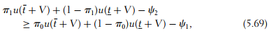
as well as the participation constraint
![]()
As usual, both constraints above are binding at the optimum of the principal’s problem. This yields the following expression of the second-best transfers: ![]()
![]() , where Δψ = ψ2 − ψ1
, where Δψ = ψ2 − ψ1
Under the agent’s ownership, the principal gets the following payoff by induc- ing a productive effort:
![]()
where

By instead offering a fixed wage t¯ = t = t, no productive effort is induced and t is chosen so that the agent’s participation constraint u(t + V) − ψ1 ≥ 0 is binding. One easily finds that
![]()
where ![]()
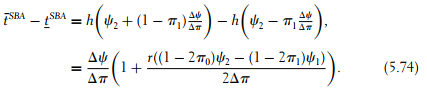
When V is large enough, the agent should own the asset in order to obtain this socially valuable proceed. The principal then induces a productive effort only when V1A > V0A, i.e., if and only if ![]() .
.
Under the assumption that tasks are substitutes, it is easy to check that C2SB − C1FB ≥ C1SB. Hence, when the agent owns the asset, inducing a productive effort becomes more costly for the principal than when the agent does not own it. The principal chooses less often to induce a productive effort than when he owns the asset himself.
However, it is worth noting that, on the condition that inducing effort remains optimal, the agent should be put under a higher powered incentive scheme when he also owns the asset. Indeed, under agent’s ownership, we have
When the principal owns the asset, the power of incentives is instead given by
![]()
The comparison of these incentive powers amounts to comparing Δψ and ψ1. For substitute tasks, the agent is thus given higher powered incentives when he owns the asset.
The intuitive explanation is as follows. Under vertical separation, the agent has greater incentives to exert effort on maintenance. The only way for the principal to incentivize the agent along the production dimension is to put him under a high- powered incentive scheme. Otherwise, the agent would systematically substitute away effort on production to improve maintenance. Asset ownership by the agent also comes with high-powered incentives akin to piece-rate contracts. Instead, less powered incentives, i.e., fixed wages, are more likely to occur under the principal’s ownership.
Holmström and Milgrom (1994) discussed the strong complemen- tarity between asset ownership and high-powered incentive schemes, arguing in a model along the lines above (but without any wealth effects), that this complementarity comes from some substitutability between efforts in the agent’s cost function of effort. They built their theory to fit a number of empirical facts, notably those illustrated by the studies of Anderson (1985) and Anderson and Schmittlein (1984). Those latter authors argued that the key factor explaining the choice between an in-house sales office and an exter- nal sales firm is the difficulty of measuring the agent’s performance. More costly measurement systems call for the choice of in-house sales. Holmström (1999b) also advanced the idea that measurement costs may be part of an explanation of the firm’s boundaries.
Source: Laffont Jean-Jacques, Martimort David (2002), The Theory of Incentives: The Principal-Agent Model, Princeton University Press.