Developed as an extension of probability theory, queuing theory deals with the analysis of congestion and delay in economic modeling.
Queuing theory features in stock control in the shape of the Lifo (Last in first out) and Fifo (First in first out) principles, and in financial markets.
Also see: information theory
Source:
D Gross and C M Harris, Fundamentals of Queuing Theory (New York, 1985)
Spelling
The spelling “queueing” over “queuing” is typically encountered in the academic research field. In fact, one of the flagship journals of the profession is Queueing Systems.
Single queueing nodes
A queue, or queueing node can be thought of as nearly a black box. Jobs or “customers” arrive to the queue, possibly wait some time, take some time being processed, and then depart from the queue.
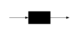
A black box. Jobs arrive to, and depart from, the queue.
The queueing node is not quite a pure black box, however, since some information is needed about the inside of the queuing node. The queue has one or more “servers” which can each be paired with an arriving job until it departs, after which that server will be free to be paired with another arriving job.
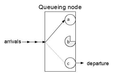
A queueing node with 3 servers. Server a is idle, and thus an arrival is given to it to process. Server b is currently busy and will take some time before it can complete service of its job. Server c has just completed service of a job and thus will be next to receive an arriving job.
An analogy often used is that of the cashier at a supermarket. There are other models, but this is one commonly encountered in the literature. Customers arrive, are processed by the cashier, and depart. Each cashier processes one customer at a time, and hence this is a queueing node with only one server. A setting where a customer will leave immediately if the cashier is busy when the customer arrives, is referred to as a queue with no buffer (or no “waiting area”, or similar terms). A setting with a waiting zone for up to n customers is called a queue with a buffer of size n.
Birth-death process
The behaviour of a single queue (also called a “queueing node”) can be described by a birth–death process, which describes the arrivals and departures from the queue, along with the number of jobs (also called “customers” or “requests”, or any number of other things, depending on the field) currently in the system. An arrival increases the number of jobs by 1, and a departure (a job completing its service) decreases k by 1.

A birth–death process. The values in the circles represent the state of the birth-death process. For a queueing system, k is the number of jobs in the system (either being serviced or waiting if the queue has a buffer of waiting jobs). The system transitions between values of k by “births” and “deaths” which occur at rates given by various values of λi and μi, respectively. Further, for a queue, the arrival rates and departure rates are generally considered not to vary with the number of jobs in the queue, so a single average rate of arrivals/departures per unit time to the queue is assumed. Under this assumption, this process has an arrival rate of λ = λ1, λ2, …, λk and a departure rate of μ = μ1, μ2, …, μk (see next figure).

A queue with 1 server, arrival rate λ and departure rate μ.
Balance equations[edit]
The steady state equations for the birth-and-death process, known as the balance equations, are as follows. Here {\displaystyle P_{n}} denotes the steady state probability to be in state n.

- {\displaystyle \mu _{1}P_{1}=\lambda _{0}P_{0}}
- {\displaystyle \lambda _{0}P_{0}+\mu _{2}P_{2}=(\lambda _{1}+\mu _{1})P_{1}}
- {\displaystyle \lambda _{n-1}P_{n-1}+\mu _{n+1}P_{n+1}=(\lambda _{n}+\mu _{n})P_{n}}


The first two equations imply
- {\displaystyle P_{1}={\frac {\lambda _{0}}{\mu _{1}}}P_{0}}

and
- {\displaystyle P_{2}={\frac {\lambda _{1}}{\mu _{2}}}P_{1}+{\frac {1}{\mu _{2}}}(\mu _{1}P_{1}-\lambda _{0}P_{0})={\frac {\lambda _{1}}{\mu _{2}}}P_{1}={\frac {\lambda _{1}\lambda _{0}}{\mu _{2}\mu _{1}}}P_{0}.}

By mathematical induction,
- {\displaystyle P_{n}={\frac {\lambda _{n-1}\lambda _{n-2}\cdots \lambda _{0}}{\mu _{n}\mu _{n-1}\cdots \mu _{1}}}P_{0}=P_{0}\prod _{i=0}^{n-1}{\frac {\lambda _{i}}{\mu _{i+1}}}.}

The condition {\displaystyle \sum _{n=0}^{\infty }P_{n}=P_{0}+P_{0}\sum _{n=1}^{\infty }\prod _{i=0}^{n-1}{\frac {\lambda _{i}}{\mu _{i+1}}}=1} leads to:

- {\displaystyle P_{0}={\frac {1}{1+\sum _{n=1}^{\infty }\prod _{i=0}^{n-1}{\frac {\lambda _{i}}{\mu _{i+1}}}}},}

which, together with the equation for {\displaystyle P_{n}} {\displaystyle (n\geq 1)}, fully describes the required steady state probabilities.

Kendall’s notation
Single queueing nodes are usually described using Kendall’s notation in the form A/S/c where A describes the distribution of durations between each arrival to the queue, S the distribution of service times for jobs and c the number of servers at the node.[5][6] For an example of the notation, the M/M/1 queue is a simple model where a single server serves jobs that arrive according to a Poisson process (where inter-arrival durations are exponentially distributed) and have exponentially distributed service times (the M denotes a Markov process). In an M/G/1 queue, the G stands for “general” and indicates an arbitrary probability distribution for service times.
Example analysis of an M/M/1 queue
Consider a queue with one server and the following characteristics:
- λ: the arrival rate (the expected time between each customer arriving, e.g. 30 seconds);
- μ: the reciprocal of the mean service time (the expected number of consecutive service completions per the same unit time, e.g. per 30 seconds);
- n: the parameter characterizing the number of customers in the system;
- Pn: the probability of there being n customers in the system in steady state.
Further, let En represent the number of times the system enters state n, and Ln represent the number of times the system leaves state n. Then for all n, |En − Ln| ∈ {0, 1}. That is, the number of times the system leaves a state differs by at most 1 from the number of times it enters that state, since it will either return into that state at some time in the future (En = Ln) or not (|En − Ln| = 1).
When the system arrives at a steady state, the arrival rate should be equal to the departure rate.
Thus the balance equations
- {\displaystyle \mu P_{1}=\lambda P_{0}}
- {\displaystyle \lambda P_{0}+\mu P_{2}=(\lambda +\mu )P_{1}}
- {\displaystyle \lambda P_{n-1}+\mu P_{n+1}=(\lambda +\mu )P_{n}}


imply
- {\displaystyle P_{n}={\frac {\lambda }{\mu }}P_{n-1},\ n=1,2,\ldots }

The fact that {\displaystyle P_{0}+P_{1}+\cdots =1} leads to the geometric distribution formula

- {\displaystyle P_{n}=(1-\rho )\rho ^{n}}

where {\displaystyle \rho ={\frac {\lambda }{\mu }}<1.}

Simple two-equation queue
A common basic queuing system is attributed to Erlang, and is a modification of Little’s Law. Given an arrival rate λ, a dropout rate σ, and a departure rate μ, length of the queue L is defined as:
- {\displaystyle L={\frac {\lambda -\sigma }{\mu }}.}

Assuming an exponential distribution for the rates, the waiting time W can be defined as the proportion of arrivals that are served. This is equal to the exponential survival rate of those who do not drop out over the waiting period, giving:
- {\displaystyle {\frac {\mu }{\lambda }}=e^{-W{\mu }}}

The second equation is commonly rewritten as:
- {\displaystyle W={\frac {1}{\mu }}\mathrm {ln} {\frac {\lambda }{\mu }}}

The two-stage one-box model is common in epidemiology.[7]
Overview of the development of the theory
In 1909, Agner Krarup Erlang, a Danish engineer who worked for the Copenhagen Telephone Exchange, published the first paper on what would now be called queueing theory.[8][9][10] He modeled the number of telephone calls arriving at an exchange by a Poisson process and solved the M/D/1 queue in 1917 and M/D/k queueing model in 1920.[11] In Kendall’s notation:
- M stands for Markov or memoryless and means arrivals occur according to a Poisson process;
- D stands for deterministic and means jobs arriving at the queue which require a fixed amount of service;
- k describes the number of servers at the queueing node (k = 1, 2, …).
If there are more jobs at the node than there are servers, then jobs will queue and wait for service
The M/G/1 queue was solved by Felix Pollaczek in 1930,[12] a solution later recast in probabilistic terms by Aleksandr Khinchin and now known as the Pollaczek–Khinchine formula.[11][13]
After the 1940s queueing theory became an area of research interest to mathematicians.[13] In 1953 David George Kendall solved the GI/M/k queue[14] and introduced the modern notation for queues, now known as Kendall’s notation. In 1957 Pollaczek studied the GI/G/1 using an integral equation.[15] John Kingman gave a formula for the mean waiting time in a G/G/1 queue: Kingman’s formula.[16]
Leonard Kleinrock worked on the application of queueing theory to message switching (in the early 1960s) and packet switching (in the early 1970s). His initial contribution to this field was his doctoral thesis at the Massachusetts Institute of Technology in 1962, published in book form in 1964 in the field of message switching. His theoretical work published in the early 1970s underpinned the use of packet switching in the ARPANET, a forerunner to the Internet.
The matrix geometric method and matrix analytic methods have allowed queues with phase-type distributed inter-arrival and service time distributions to be considered.[17]
Systems with coupled orbits are an important part in queueing theory in the application to wireless networks and signal processing. [18]
Problems such as performance metrics for the M/G/k queue remain an open problem.[11][13]
Service disciplines

First in first out (FIFO) queue example.
Various scheduling policies can be used at queuing nodes:
- First in first out
- Also called first-come, first-served (FCFS),[19] this principle states that customers are served one at a time and that the customer that has been waiting the longest is served first.[20]
- Last in first out
- This principle also serves customers one at a time, but the customer with the shortest waiting time will be served first.[20] Also known as a stack.
- Processor sharing
- Service capacity is shared equally between customers.[20]
- Priority
- Customers with high priority are served first.[20] Priority queues can be of two types, non-preemptive (where a job in service cannot be interrupted) and preemptive (where a job in service can be interrupted by a higher-priority job). No work is lost in either model.[21]
- Shortest job first
- The next job to be served is the one with the smallest size
- Preemptive shortest job first
- The next job to be served is the one with the original smallest size[22]
- Shortest remaining processing time
- The next job to serve is the one with the smallest remaining processing requirement.[23]
- Service facility
- Single server: customers line up and there is only one server
- Several parallel servers–Single queue: customers line up and there are several servers
- Several servers–Several queues: there are many counters and customers can decide going where to queue
- Unreliable server
Server failures occur according to a stochastic process (usually Poisson) and are followed by the setup periods during which the server is unavailable. The interrupted customer remains in the service area until server is fixed.[24]
- Customer’s behavior of waiting
- Balking: customers deciding not to join the queue if it is too long
- Jockeying: customers switch between queues if they think they will get served faster by doing so
- Reneging: customers leave the queue if they have waited too long for service
Arriving customers not served (either due to the queue having no buffer, or due to balking or reneging by the customer) are also known as dropouts and the average rate of dropouts is a significant parameter describing a queue
I¦ve recently started a website, the information you provide on this web site has helped me tremendously. Thanks for all of your time & work.
Attractive section of content. I just stumbled upon your website and in accession capital to assert that I acquire actually enjoyed account your blog posts. Anyway I will be subscribing to your augment and even I achievement you access consistently rapidly.