In the remainder of this chapter we report and analyze certain results of a simulation experiment using the model. This experiment is a p reliminary exploration of the influence of initial market structure on the innovative and price performance of the industry and on the evo lution of industry structure over time. Other experiments that are fo cused on particular issues, some of which come into view as a result of this set of runs, are discussed in the following two chapters.
In the simulations reported here, five different sets of initial con ditions were examined, with two, four, eight, sixteen, and thirty two firms in the industry. In each condition half of the firms spend on R&D for innovation as well as for imitation, and the other half spend only on imitative R&D. For any given setting all the firms are of equal size initially and have the same productivity level, which is equal to the level of latent productivity. While all firms have the same initial production costs, the firms that spend on innovative as well as imitative R&D have higher total costs per unit of output, at least ini tially. The initial total capital stock (and the stocks of each firm) were chosen so that, for each initial structure, desired total net i nvestment was zero. Since a smaller margin over production cost induces posi tive i nvestment when a firm’s market share is small compared to when it is large, this means that total cap ital is larger initially and initial price is lower, the larger the number of firms. The levels of rin and rim are adjusted to compensate for the difference in initial capital, so that the initial levels of total innovation expense and total imita tion expense are the same in all runs. Thus, the initial expected val ues of innovation draws and imitation draws are the same under all initial conditions; in this sense, the industry is initially equally pro gressive under all initial conditions.
In addition to differences in the number of firms and in initial in dustry output and price, we also explored differences between two regimes of finance for firm investment. Under one regime a firm can borrow up to 2.5 times its own net profits for financing investment. Und er the other regime, firm’s borrOWings were limited to a matching of their profits.
Thus, there are ten experimental conditions in all- five market structures times two financial regimes. Each condition was run five times. The runs lasted 101 p eriods e ach -l00 periods after initial conditions. For the particular parameter values chosen, a period can be thought of as corresponding to a quarter of a year; hence, the com puter runs are of twenty-five years .
The runs here relate to an industry with science-based technology in which latent productivity advances at 1 percent a quarter or 4 per cent a year. Values of rin for the innovative firms correspond to an R&D-sales ratio of about . 12, which by empirical standards is high. This high value was chosen so that the cost of doing innovative R&D would stand out clearly in the initi al experiments. The probability of innovative R&D success was set so that the industry as a whole averaged about two innovative finds per year, at initial conditions. And at initial conditions, an imitation draw was about as likely for the industry as a whole as an innovative draw.
The elasticity of demand for the industry’S product was set equal to one. This is an important fact in understanding the simulation runs, since it meant that total capital in the industry tended to stay relatively constant over the runs. Growing productivity meant falling prices and growing output, but relatively constant input (in this case, capital input), As a result, the average number of imitation draws per p eriod tended to be roughly constant over the run. The average number of innovative draws tended to grow or decline as the share of industry capital accounted for by innovators grew or declined.
With the vision of hindsight, we know that the parameter settings for this particular set of runs- in particular, the rate of growth of la tent productivity, the productivity of innovative R&D in terms of the probability of finding a new technique per dollar of expenditure , and the productivity of imitative R&D expenditure in terms of the proba bility of successful imitation per dollar- defined a regime in which innovative R&D is somewhat unprofitable on average. In Chapter 14 we will explore the conditions that determine whether or not innova tive R&D is profitable and the difference it makes to overall industry performance. But here, keeping in mind that the climate is not favor able to innovative R&D, we can ask two sets of questions.
First, how does industry performance over a considerable number of periods depend on the initial concentration of the industry? There are several different performance variables worth examining. One is the time path of the best practice (highest productivity) in the in dustry. Another is the time path of average practice (average produc tivity). Also, it seems important to consider the effect of initial con centration on the average markup over production costs in the industry. And, finally, what happens to the price is obviously of con siderable interest.
Second, it is interesting to explore the effects of initial concentration on the way in which industry structure evolves over time. In this context, where innovative R&D is not profitable, in what way does the survivability of firms that do innovative R&D depend on initial concentration? More generally, which initial structures tend to be stable and which unstable? Do the initially unconcentrated struc tures tend to concentrate over time? Do the initially concentrated structures tend to concentrate further?
These are the kinds of questions we will be exploring. Our prelim inary answers will sharpen intuition regarding the processes of dynamic competition in our model industry and raise some specific questions that we will explore in subsequent runs.
1. Performance
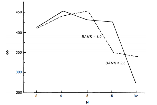
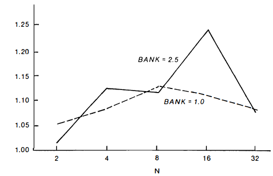
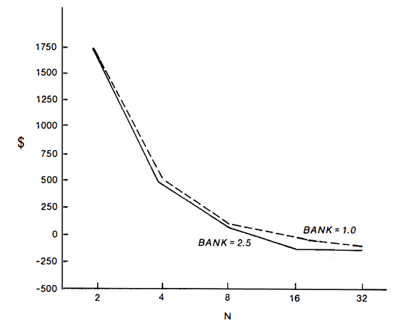
Figures 12.1-12.6 show various performance variables as a function of initial structure. The solid line shows pverage performance of the five runs in which the firms had considerable access to bank credit (BANK = 2.5). The dotted line shows average performance when bank credit was more limited (BANK = 1.0). All values shown are at the end of the run and are means over five runs.
Figure 12.1 shows best-practice productivity in period 101. In this model the evolution of best practice (or at least best practice at the end of the run) does not appear to depend upon initial concentration.
Figure 12. 2 shows average productivity at the end of the run as a function of initial concentration. Figure 12.3 shows the “average pro-ductivity gap” defined as th e geometric mean over time of the ratio of average productivity to latent prod uctivity, minus one. Both of these indices show that average productivity toward the end of the run (and apparently over a considerable part of the run) was lower when there were many firms than when there were few. Thus, the small-numbers cases were marked by a considerably higher ratio of average productivity to best- practice productivity than were the large-numbers cases. Since the initial productivity levels of all firms were the same under all initial conditions, average productivity apparently rose m ore rapidly and average production costs declined more rapidly in the small- numbers cases than in the large-numbers cases.
While this latter result is consistent with the Schumpeterian hy pothesis, the fact that growth of best- practice productivity ap parently is invariant to initial industry structure suggests that some thing different might be going on. Figure 12.4 displays cumulative innovative R&D expenditure over the course of the run, for the dif ferent initial market structures. Neither end-period best- practice productivity nor average-practice productivity seems well correlated with innovative R&D outlays of the industry.
That the evolution of best- practice productivity is not strongly sensitive to total industry innovative R&D expenditures or to in-dustry struc ture can be partially explained as follows . In the version of the model under exploration here, the driving force of tech nological advance in the industry is growth of latent productivity I which is occurring as a result of forces exogenous to the actions of the firms in the industry. The innovative R&D efforts of the firms in the industry take advantage, as it were , of new technological opportuni-ties that have been created elsewhere. Greater R&D expenditure within the industry means that latent productivity is tracked more smoothly, but aside from that the path of best-practice productivity is unlikely to be much higher than it is when industry R&D expendi tures are less. In the situation explored in these runs, which we have called the “science-based industry” case, there are sharply dimin ishing returns to industry R&D expenditure. The situation might be quite different when there is no exogenous growth of technological opportunities and when technological advance in the industry builds on itself-what we call the “‘cumulative technology” case. We shall explore the differences in Chapter 14. However, it is apparent that in the particular runs considered here, enough innovative R&D was going on even in the runs of sixteen and thirty-two firms so that la tent productivity is being tracked reasonably well by best practice.

12.1 Best-practice prod uctivity.

12.2 Average productivity

12.3 Average productivity gap
12.4 Cumulative expenditure on innovative R&D.
Why, then, is average productivity so sensitive to industry struc ture? The answer relates, ultimately, to the particular view of the na ture of the firm that is implicit in our model-that is, to the theoreti cal significance of the firm as an institution. Within the boundaries of a firm, technical information that is available for use with one unit of capital is equally and costlessly applicable to all other units. On the other hand, scarce resources are consumed by the innovation and imitation processes that first bring new information into the firm. No doubt this contrast is overdrawn in our modeC as theoretical co n trasts usually are. But it is certainly broadly consistent with the view of the firm that we set forth in Part II.
More specifically, the effect on average productivity arises in the following way. Innovative R&D effort yields, from time to time, superior techniques that temporarily define “best practice.” The larger the innovator relative to the industry, the larger the immediate effect of such a technical change on industry average productivity. Similarly, when a new technique is imitated, the larger the imitator relative to the industry, the larger the impact on industry average productivity of each successive imitation of the new technique. In the model, the rate at which acts of imitation (imitation draws) occur is roughly independent of industry structure. Thus the lessening of the effect of each individual draw, because of the smaller amount of capital affected when the number of firms is larger, is fully reflected in industry average productivity. For a given level of industry expenditure on innovative R&D, the productivi ty level associated with best-practice technique is independent of industry structure. But the gap between average and best-practice productivity is larger in the more fragmented structure because of the reduced scope of ap plication of individual successes in innovation and i mitation.
Since there will always be at least one innovating firm among those that have the best-practice productivi ty level at a given time, one might expect that a widening gap between best practice and average productivity would be associated with a widening gap between the average productivity of innovators as compared to imi tators. Figure 12.5 shows that this expectation is borne out-up to a point. But the innovatorsl superiority in productivity is smaller in the case of thirty-two firms than it is in the eight-firm case. This re sult presumably reflects the fact that the selection forces are operating strongly against the innovators in the thirty-two-firm case. A small innovative firm that has not actually had a success recently is more likely to be using out-of-date techniques than is a larger i mita tor that successfully plays the IIfast secondll strategy.
Thus, in this model a more competitively structured indus try does lead to a poorer productivity performance than does an industry that is more concentrated. But the reason is not the one commonly asso ciated with the Schumpeterian hypothesis: that best-pricatice tech nology evolves more slowly in the many-firm case than in the few firm case. It is that there is a much larger gap between best practice and average practice in the case where industry capital is fragmented than there is in the case where it is concentrated.
While average production costs are higher in the many-firm case, Figure 12.6 shows that the average price-cost margin is lower where industry structure is more competitive. Figure 12.7, which displays total net worth, shows the same thing: the excess-profit rate (and net worth) is higher when the industry starts concentrated than when it starts unconcentrated. The reason is right out of the textbooks: per ceived market power associated with larger market shares has led to investment restraint and thus to higher prices and profit margins.
12.5 Ratio of average productivity: innovators/imitators.

12.6 Percentage margin over average cost
12.7 Total net worth
Figure 12 .8 shows end-of-run price in the industry as aU-shaped function of the number of firms. Up to a point, in these runs at least, the lower margin, which is associated with more competitive struc ture, more than offsets the higher unit production costs. However, the curve appears to turn upward as the industry gets very competi tive. Beyond eight firms, the additional competition yields only lim ited gains in terms of lower margins, and further deconcentration en tails costs in terms of lower average productivity.
2. Evolution of Structure
We already have remarked that the parameter settings of these runs define a context in which innovative R&D is not profitable. Figure 12.9 presents the research expense recovery rate. This is a simple descriptive measure of the extent to which firms that do innovative R&D recapture, in transient profits derived from superior productiv ity, the funds they spend on R&D. The measure is defined as the dif ference between the final net worths of innovators and imitators, divided by cumulative R&D expense, plus one. The value of 1.0 cor responds, obviously, to a case in which the final net worths of inno-vators and imitators are equal. In this case the productivity advan tages gained from innovative R&D are worth j ust enough to be offset by the cost of R&D. A value of 0.5 indicates that the pecuniary ben efit that innovators derive from their R&D amounts to only half of what they spend. Figure 12.9 shows that, in general, innovative R&D does not pay in these runs. The net worth differences between inno vative firms and firms that do no innovative R&D are displayed in Figure 12.10. Essentially they mirror the results of the previous figure.


A straightforward application of the selection argument would lead one to expect, given the profitability differential, that the firms that undertook innovative R&D would be driven out of business. Figure 12.11 shows that this is too simple. Despite their relative un profitability compared with firms that did only imitative R&D, in the small- numbers cases the innovators accounted for more than half of the industry’S capital stock toward the end of the run. Only in the thirty-two-firm case was the unprofitability of innovative R&D clearly reflected in the innovators’ capital share.
It is apparent that this is the consequence of two factors. First, in the small-numbers cases competition among firms was sufficiently restrained so that, even though the innovators were not as profitable as the imitators, they still made positive profits . The reluctance of large profitable firms to expand their capital stock and thus “spoil the market” prOVided a shelter for firms that were less profitable. Sec-ond, we have assumed in this model that a firm’s desire to expand its capacity for production is tied to the margin between prices and pro duction costs. For two firms with the same market share, the firm with the lower production cost will have a higher target output and capital stock than the firm with the higher production cost, even though including R&D expenditures the former may have higher total cost per unit of output than the latter. When profits are high, there is no financial constraint to prevent the difference in targets from being reflected in reality.


The latter mechanism is the explanation for the fact that the inno vators’ capital share actually exceeds 0.5 in most of the runs. But on the more basic issue of the survival of the innovators, it is the invest ment restraint associated with the concentrated structure that is the key. If the more profitable firms were more aggressive in expanding their capacity even when they were large, it appears that the firms that did innovative R&D would indeed be gradually run out of busi ness. The consequences of this might not be too serious if the evolu tion of technology in the industry were science-based, as in the runs here, but it might be serious if the technological regime were cumu lative. We shall explore these questions in a later chapter.
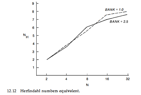
What can one say about the evolution of economic structure more generally? While runs that started out with a highly concentrated market structure tended to remain concentrated, there was a marked increase in concentration in the runs with an unconcentrated initial structure. Figure 12.12 displays end-of-run values of the “Herfindahl numbers equivalent.” This is a meas ure of output concentration in the industry; intuitively it is the number of firms in an i ndustry of equal-sized firms that has the same degree of concentration as the actual industry according to the Herfindahl-Hirschman measure. Thus, the fact that the numbers equivalent is very cl ose to 2 .0 in all the duopoly cases is a reflection of the fact that the two firms do re main very nearly equal in size in these cases. In the four-firm cases, there is a slight tendency for concentration to increase over the run. This tendency becomes pronounced beginning with the eight-firm cases . In the ten runs with thirty-two firms, the largest final value for the numbers equivalent is a level of concentration comparable to the consequences of the disappearance of well over half of the firms ini tially in business, if the remainder were of equal size. And , as we have seen above, the bulk of the concentration increase involved the decline of firms who had policies of investing in innovative R&D.
In this chapter we have explored the behavior of our mod el of Schumpeterian competition with various initial industry structures in a context where, in general, innovative R&D was not profitable. We considered both how industry performance was influenced by initi al industry structure, and how industry structure evolved over time. In Chapter 13 we will co nsider in more detail questions relating to the evolution of i ndustry structure. In Chapter 14 we will consider in more detail the structure-performance links.
Source: Nelson Richard R., Winter Sidney G. (1985), An Evolutionary Theory of Economic Change, Belknap Press: An Imprint of Harvard University Press.