The computer output describing the experimental simulation runs contains abundant quantitative detail and is rich in qualitative pat terns . Firms thrive and decline; new techniques appear, dominate the scene briefly, and then fade away. Time series for most aggregate data display strong trends, and also a good deal of short-period fluc tuation. The stack of paper containing the description of the total of eight hundred years of synthetic history is over eight inches high. It is clear that it must be summarized fairly dras tically for the purpose of this discussion.
How do the aggregative time series look? In a word, plausible. In Table 9.1 the results of one simulation run and the real data ad dressed by Solow are displayed side by side. There is, of course, no reason to expect agreement between the real and simulated data on a year-to-year basis. The simulation run necessarily reflects nonhis-torical random influences. But more than that, and of particular im portance to this comparison, the simulation model, unlike Solow’s analysis of the real data, generates its own input history on the basis of very simple assumptions about behavior and institutional struc ture . The real period in question involved eposides of economic de pression and war, and while these episodes might be considered as historical random events, the simulation model is not p repared to deal with them realistically. The same trend in the labor force, the same Say’s Law assumption, the same link of investment to retained earnings persist year by year. Since the model’s historical accuracy is so sharply limited by these considerations we have not attempted to locate parameter settings that would, in any sense, maximize simi larity to the real time series. For example, it would have been easy to assure a better match of initial conditions.


Rather, the question we thi nk should be addressed is whether a behavioral-evolutionary model of the economic growth process, of the sort described in the preceding section, is capable of generating (and hence of explaining) macro time series data of roughly the sort actually observed. So considered, we regard the simulation as quite successful . The historically observed trends in the output-labor ratio, the capital-labor ratio, and the wage rate are all visible in the simu lated data. The column headed A in the table shows the Solow-type index o'{ technology, computed on the contrafactual assumption that the simulated time series were generated by a neutrally shifting neo classical pro duction function. The simulated average rate of change in this measure is about the same as in the Solow data (indicating, essentially, that we have chosen an appropriate value in this run for our localness-of- search parameter). It is interesting to note, however, that our simulated world of diverse simple-minded firms searching myopically in a continuing disequilibrium generates a somewhat smoother aggregate “technical progress” than that found by Solow in the real data for the United States. For example, our series shows only five incidences of negative technical progress, whereas Solow’s series shows eleven- and the run shown is typical in this respect.
Table 9.2 presents d ata on each run for each of several variables, observed at period forty of the run.4 Also displayed are the corre sponding figures, where these exist, for the thirty-sixth period (1944) and the fortieth period (1948) of the Solow data. Given the experi mental design, it is convenient to distinguish the runs by numbering them in the binary system. The interpretive key to this numbering is explained in the note to Table 9.2.
It is plain that the simulation model does generate “technical progress” with ri sing output per worker, a rising wage rate, and a rising capital-labor ratio, and a roughly constant rate of return on capital . The rates of change produced correspond roughly to those in the Solow data. Also, some individual runs produce values quite close to the Solow values for the variables measured -for example, runs 0101 and 0111.

Figures 9.2-9.5 display the time paths of the average input coefficients generated by the sixteen runs. To keep the figures relatively uncluttered , the values are plotted for the initial period and at periods 5, la, and so on thereafter. In Figure 9.6 the input coefficient track for one run (11 10) is compared with the track implied in the Solow data. The case shown is one in which there is close agreement at the initial point, and also forty periods later, but there is a wide di vergence in between. The divergence is associated with the fact that, while the simulated track gives the impression of taking a relatively constant direction, there is a sharp turn in the track of the real data, suggestive of a change in the underlying regime. The apparent break occurs between 1929 and 1934 . Perhaps it would be asking too much of the simulation model, committed as it is to fu. ll employment, to reproduce that b reak.
It seems interesting to ask: If a neoclassical economist believed the aggregative time saving generated by the simulation model to be real data, and tested his theory against the data, what would he conclude?

9.2 Average input coefficient paths for four runs with low emphasis on imi tation and no bias in search.

9.3 Average input coefficient paths for four runs with high emphasis on imitation and no bias in search.

9.4 Average input coefficient pa ths for four runs with low emphasis on imi tation and labor-saving bias in search.

9.5 Average input coefficient paths for four runs with high emphasis on imitation and labor- saving bias in search.
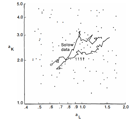
9.6 Average input coefficient pa ths: Solow data compared with run 1111

The answer depends on the particular simulation run from which the data are taken and on the particular test. But by and large it seems that he would believe that his theory had performed well. (Of course, if he also looked at the microeconomic data and observed the inter firm dispersion of techniques and differential growth rates, he might ponder a bit whether his theory really characterized what was going on. But the pondering would likely conclude with the consoling thought that macro theories need not square with micro observa tions.)
Tables 9.3 and 9.4 display the results of fitting Cobb-Douglas pro duction functions, by each of two methods, to the aggregate time series data for each experimental run. The Solow procedure was fol lowed in generating Table 9.3 . The percentage neutral shift in the hypothetical aggregate production function was calculated in each period, and the technology index A(t) constructed . The index was then employed to purge the output data of technological change, and the log of adjusted output per labor unit was regressed on the log of capital per labor unit. The observations were taken from periods 5-45 of the simulation run, to give us a sample size the same as Solow’s and to minimize possible initial- phase and terminal-phase effects on the outcomes. The regressions in Table 9.4 are based on an assumed exponential time trend in the technology index and involve the logs of the absolute magnitudes rather than ratios to labor input. The same sample period was employed.

The most noteworthy feature of these results is that the fits ob tained in most of the cases are excellent: half of the R2 values in Table 9.3 exceed 0. 99, and more than half of those in Table 9.4 equal 0. 999 . The fact that there is no production function in the simulated economy is clearly no barrier to a high degree of success in using such a function to describe the aggregate series it generates. It is true that the fits obtained by Solow and others with real data are at least as good as most of ours, but we doubt that anyone would want to rest a case for the aggregate production function on what happens in the third or fourth decimal place of R2. Rather, this particular contest between rival explanatory schemes should be regarded as essentially a tie, and other evidence consulted in an effort to decide the issue.
Thus, a model based on evolutionary theory is quite capable of generating aggregate time series with characteristics corresponding to those of economic growth in the United States. It is not reasonable to dismiss an evolutionary theory on the grounds that it fails to pro vide a coherent explanation of these macro phenomena. And the explanation has a certain transparency. As we discussed earlier, many of the familiar mechanisms of the n eoclassical explanation have a place in the evolutionary framework.
Consider, for example, the empirically observed nexus of rising wage rates, rising capital intensity, and increasing output per worker. Our simulation model generated data of this sort. In that model, ,as in the typical neoclassical one, rising wage rates provide signals that move individual firms in a capital-intensive direction. As was proposed in Chapter 7, when firms check the profitabili ty of alternative techniques that their search processes uncover, a higher wage rate will cause to fail the “more profitable” test certain tech niques that would have “passed” at a lower wage rate, and will enable to pass the test others that would have failed at a lower wage rate. The former will be capital-intensive relative to the latter. Thus, a higher wage rate nudges firms to move in a capital- intensive direc tion compared with that in which they would have gone. Also, the effect of a higher wage rate is to make all technologies less profitable (assuming, as in our model, a constant cost of capital), but the cost increase is proportionately greatest for those that display a low capital-labor ratio; thus, a rise in wages tends to increase industry capital intensity relative to what would have been obtained. And output per worker will be increased; a more capital-intensive tech nology cannot be more profitable than a less capital- intensive one unless output per worker is higher.
While the explanation here has a neoclassical ring, it is not based on neoclassical premises. Although the firm s in our simulation model respond to profitability signals in making technique changes and investment decisions, they are not maximizing profits. Their behavior could be rationalized equally well (or poorly) as pursuit of the quiet life (since they relax when they are doing well, and typi cally make only small changes of technique when they do change) or of corporate growth (since they maximize inves tment subject to a payout constraint). Neither does our model portray the economy as being in equilibrium. At any given time, there exists considerable diversity in techniques used and in realized rates of return. The ob served constellations of inputs and outputs cannot be regarded as optimal in the Paretian sense: there are always better techniques not being used because they have not yet been found and always laggard firms using technologies less economical than current best practice. On our reading, at least, the neoclassical interpretation of long run productivity chan ge is sharply different from our own. It is based on a clean distinction between “moving along” an existing production function and shifting to a new one. In the evolutionary theory, substitution of the II search and selection” metaphor for the maximization and equilibrium metaphor, plus the assumption of the basic improvability of procedures, blurs the notion of a production function. In the simulation model discussed above, there was no production function-only a set of physically possible activities. The production function did not emerge from that set because it was not assumed that a p articular subset of the possible techniques would be “known” at each particular time. The exploration of the set was treated as a historical, incremental process in which nonmarket in formation flows among firms played a maj or role and in which firms really “know” only one technique at a time. We argue-as others have before us- that the sharp “growth accounting” split made within the neoclassical paradigm is bother some empirically and conceptually. Consider, for example, whether it is meaningful to assess the relative contribution of greater mechan-ization versus new technology in increasing productivity in the tex tile industries during the Industri al Revolution, of scale economies versus technical change in enhancing productivi ty in the generation of electric power, or of greater fertilizer usage versus new seed varieties in the increased yields associated with the Green Revolu tion . In the Textile Revolution the major inventions were ways of substituting capital for labor, induced by a si tuation of growing labor scarcity. It could plausibly be argued that in the electric power case, various well-known physical laws implied that the larger the scale for which a plant was designed, the lower the cost per unit of output it should have. However, to exploit these latent possibilities required a considerable amount of engineering and design work, which became profitable only when the constellation of demand made large- scale units pl ausible. Plant biologists had long known that certain kinds of seed varieties were able to thrive with large quantities of fertilizers and that others were not. However, until fer tilizer prices felt it was not worthwhile to invest significan t resources in trying to fi nd these varieties. In all of these cases, pat terns of demand and supply were evolving to make profitable dif ferent factor proportions or scales. But the production set was not well defined in the appropriate direction from existing practice. It had to be explored and created.
We argued in Part II that at any given time the set of techniques that an individual c a’n control skillfully, or that an organization can control routinely, likely does not extend very far beyond those that are being more or less regularly exercised. Relatedly, we proposed that an attempt · to employ a technique significantly different from those likely involves a nontrivial amount of deliberation, research, trial and feedb ack, and innovation. But in Chapters 6 and 7, and here again, models in which only a small part of changed input-output re lations could be regarded as “routine” (moving along a production function) displayed patterns over time that had many of the qualita tive properties of movements along the production functions of orthodox theory. The model in this chapter is somewhat extreme in endowing a firm with only one technique that it can operate rou tinely at any time. It would not be inconsistent with evolutionary theory to assume that a firm at any time is capable of operating a small number of alternative techniques, with various decision rules employed to determine the mix. In this case a larger share of factor substitution in response to changing prices would have been ac counted for by along-the-rule movements. But it is interesting that even with along-the-rule responses excluded completely, an evolu tionary model is capable of generating, and hence explaining, data that orthodox theory explains only by recourse to the unrealistic as-sumption that firms have large, well- defined production sets that ex tend well beyond the experienced range of operation.
The question of the nature of “search” processes would appear to be among the most important for those trying to understand eco nomic growth, and the evolutionary theory has the advantage of posing the question explicitly. In the simulation model, we assumed that technical progress was the result strictly of the behavior of firms in the “sector” and that discovery was relatively even over time. However, it is apparent that the invention possibilities and search costs for firms in particular sectors change as a result of forces ex ogenous to the sector. Academic and governmental research certainly changed the search prospects for firms in the electronics and drug in dustries’ as well as for aircraft and seed producers. In the simulation, the “topography” of new technologies was relatively even overtime. However, various studies have shown that often new oppor tunities open up in clusters. A basic new kind of technology becomes possible as a result of research outside the sector. After a firm finds, develops, and adopts a version of the new technology, a subsequent round of marginal improvements becomes possible. This appears to be the pattern, for example, in the petroleum-refining equipment and aircraft industries. However, this pattern does not show up in the manufacture of cotton textiles (after the Industrial Revolution) or in the automobile industry, where technical advance seems to have been less discrete. The search and problem- solving orientation of an evolutionary theory naturally leads the analyst to be aware of these differences and to try somehow to explain or at least characterize them.
The perspective on the role of the “competitive environment” is also radically different in the evolutionary theory, and leads one to focus on a set of questions concerning the intertwining of competi tion, profit, and investment within a dynamic context. Is the invest ment of a particular firm strictly bounded by its own current profits? Can firms borrow for expansion? Are there limits on firm size, or costs associated with the speed of expansion? Can new firms enter? How responsive are “consumers” to a better or cheaper product? How long can a firm preserve a technically based monopoly? What kind of institutional barriers or e ncouragements are there to imita tion? The answers to these questions are fundamental to under-standing the workings of the market environment. The specifics of their treatment, like that of the nature and topography of “search, ” is an empirical issue within our theory.
These kinds of questions can be illuminated by some of the find ings of the vast literature on the micro aspects of technological change. Chapter 11 will be concerned specifically with such an explo ration. However, some interesting micro-macro links appear in our simulation model.
Source: Nelson Richard R., Winter Sidney G. (1985), An Evolutionary Theory of Economic Change, Belknap Press: An Imprint of Harvard University Press.