The task now becomes one of selecting a set of variables that permits us to translate management’s objective function into mathematical terms. This requires that two new variables be defined: (1) the fraction of actual profits that is reported and (2) staff. The first of these is necessary in order to identify the management slack absorbed as cost component. The second is essential because the staff and production decisions, contrary to the standard theory of the firm, are no longer made symmetrically. With these two exceptions, all the variables entering the model are conventional ones. Thus, the variables we consider are:

S ≡ “staff” (in money terms)
C ≡ production cost = C ( X )
ρ ≡ the fraction of actual profits reported (and (1 — ρ) is the fraction of the actual profits absorbed as cost)
ε ≡ the condition of the environment, a demand shift parameter
T ≡ taxes where t = tax rate and Ţ = lump sum tax
Second order (stability) conditions are satisfied by assuming both wellbehaved cost and revenue functions and diminishing marginal utility characteristics in the utility function.
As proposed above, the components of the objective function can be reduced to three: (1) staff ( S ), (2) management slack absorbed as cost (π A — π R ), and (3) discretionary spending on investments ( I D ). If we let U be the utility function, management’s objective becomes:
![]()
It turns out that both constraints are redundant so that both can be ignored in the subsequent analysis and the problem becomes one of finding an unconstrained maximum. Thus, the problem is to

additive in each of the terms. Thus the objective would be to

Since it is unnecessary to restrict the form of the utility function in order to obtain our results, the more general formulation is to be preferred.
24 That the first constraint is redundant is due to the fact that it takes exactly the same form as the last term in the utility function. Thus, whenever the constraint becomes binding (i.e., satisfied as an equality), the third term in the utility function itself goes to zero and with diminishing marginal utility characteristics (and assuming no corner solutions), the marginal utility becomes infinite. Given this property, the firm will, so long as it is possible, choose values for its decision variables that maintain positive values for I D (i.e., satisfy the constraint as an inequality). Thus, as the condition of the environment becomes increasingly more severe, the firm will converge to profit-maximizing behavior independent of the constraint. That the second constraint is redundant obtains from first-order conditions that require that the second and third terms in the utility function bear positive proportional relationships to one another. The analysis, however, is not dependent on the fact that both constraints are redundant. Had this not been true, the resulting inequality-constrained maximization problem could have been handled by making use of the Kuhn-Tucker theorem. All of our results would be preserved as long as the constraints were not binding.
The following first-order results are obtained by taking partial derivatives of U with respect to X, S, and ρ

From Eq. (3) it follows that ρ will be chosen so as to preserve a positive proportional relationship between the amounts of management slack absorbed as cost and discretionary spending on investments. Thus, only in the limiting case when the environment is so severe as to drive both these slack type activities to zero will ρ be chosen equal to one. Otherwise, values of ρ less than unity will be selected. Substituting Eq. (3) into Eq. (2) yields

The corresponding profit-maximizing relationships are

and ρ chosen identically equal to unity. Hence, only for the production decision do we obtain results for the behavioral model that are consistent with profit-maximizing behavior. That is, whereas the profit-maximizing firm employs staff at the level where the marginal value product equals the marginal cost of the factor (i.e., ∂ R /∂ S = 1), the behavioral firm ordinarily employs staff in the region where the marginal value product is less than the marginal cost (i.e., ∂ R /∂ S □ 1). Moreover, only under conditions where U 1 = 0 or when the firm is confronted with severe adversity (so that U 2 takes on very large positive values) will the profit-maximizing choice of staff obtain under the behavioral model. Since a value of U 1 = 0 requires an elimination of the staff term from the utility function entirely, this possibility can be ignored. Also, since by hypothesis we are dealing with firms for which economic pressures are not continuously severe, the second condition under which profit- maximizing rules would determine the staff employment decision can be treated as the unusual rather than the normal situation.
Only when the behavioral firm is confronted by conditions of economic adversity that would cause it to employ staff profit-optimally will ρ be chosen equal to one. In all other circumstances it will choose values of ρ less than unity; i.e., it will absorb some fraction of actual profits as nonproductive cost.
The fact that the behavioral model shows the production decision being made along lines consistent with profit maximization while the staff decision is not warrants further examination. This result flows directly from our assumption that staff is valued by the managers for reasons apart from productivity whereas (by implication) the only satisfaction that management derives from employing labor is that associated with the productive value of this resource. Indeed, by introducing a staff term into the utility function as we have, this result follows deductively. However, the result also accommodates itself to our observations of the business enterprise. Thus, given favorable economic conditions, staff expenditures (for selling expense, research and development, community relations, and so forth) are typically permitted to absorb large amounts of the uncommitted resources that the firm is generating. In the behavioral model, this derives from the managerial rewards associated with such expenditures — namely, from the relation these expenditures bear to salary, prestige, flexibility, and job security.
Given these equilibrium conditions, how do the decision variables adjust to a change in the parameters — to a displacement of equilibrium? 27 In particular, how does the system adjust to a change in the condition of the environment (the demand shift parameter ε), a change in the profit tax rate ( t ), and a lump sum tax (Ţ)?
It will facilitate the argument to compact the notation and designate each decision variable by X and each parameter by θ j. Then the function U ( X, S, ρ; ε, t, Ţ can be represented as U ( X 1, X 2, X 3 ; θ 1, θ 2, θ 3 ). The general form for determining the response of the pth decision variable to a change in the m th parameter becomes

where C ip is the cofactor of the ith row and p th column of D and □ D □ is the determinant of the second partials

The results for a displacement by each of the parameters are summarized in Table 9.1. The direction of adjustment of any particular decision variable to a displacement from its equilibrium value by an increase in a particular parameter is found by referring to the row and column entry corresponding to this pair.
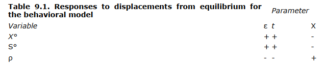
The significance of these responses can best be discussed by comparing them to the corresponding results obtained for the profit-maximizing model. These are shown in Table 9.2.

The qualitative differences between the two models are substantial. Thus, whereas the profit-maximizing firm chooses values for ρ° identically equal to one, the behavioral firm chooses values for ρ° less than unity and adjusts the value of ρ in response to a parameter change. More important are the tax effects. Whereas the profit-maximizing firm responds to neither a profit tax rate nor a lump sum tax, the behavioral firm adjusts both its output and staff decisions (as well as its choice of ρ) when taxes are changed.
Both models predict that the output and staff will be increased in response to an increase in the demand shift parameter (ε). However, the behavioral model also indicates that the fraction of profits reported will be reduced (i.e., the fraction of profits absorbed as cost will increase). Thus the management slack absorbed as cost will increase not only absolutely but also relatively as the demand for the firm’s products increases (and a deterioration of the environment will lead to a reversal of these profit absorption activities). The behavioral model therefore predicts that expenditures for travel, expense accounts, office improvements, and so forth will be very much a function of business conditions. 29 Implicitly, the profit-maximizing model denies that such a relationship should exist.
With respect to an increase in the profit tax rate, our model predicts that the firm will shift out of profits and into staff and output as well as managerial superfluities as the penalty associated with reporting profits is increased. In the presence of an excess profits tax, for example, the behavioral firm will increase expenditures on advertising, customer services, public relations, and so forth and at the same time increase the proportion of management slack absorbed as cost. Under the profit- maximizing hypothesis, however, the optimum choice of factors is unaffected by a rate increase; it therefore predicts that there will be no response to any change in the profits tax rate. Although it is possible to interpret our experience with excess profits taxes in a manner somehow consistent with a “long-run” version of profit maximization, at the level of the models we are considering here the gross evidence clearly conforms to that predicted by the behavioral model and contradicts that predicted by the profit-maximizing model.
When a lump sum tax is levied, the behavioral firm is no more able to avoid it than is the traditional firm. Since the traditional firm is already maximizing profits, it continues its operations unchanged. However, the behavioral firms, which are operating in a region that is suboptimal from the profit-maximizing standpoint, revise their strategies so as to maintain a balance between their rewards and move their decision variables in a direction that increases profits. Thus, staff, output, and the amount of management slack absorbed as cost are all reduced as the lump sum tax is increased. It might be noted that the lump sum tax is really doing triple duty inasmuch as its effect is identical to that of increasing the minimum profit constraint or imposing any sort of fixed charge on the firm. That is, the behavioral model predicts that, contrary to the traditional theory (but perhaps more in accord with standard business practice), fixed costs do influence the firm’s choice of an optimum configuration of variable factors.
Although the property does not derive from the comparative statics of our model, the fact that a newly installed executive with the assigned objective of reducing costs can remove staff with ease is an event that is entirely consistent with the behavioral model. The explanation requires only that we recognize that the objective of cost reduction implies a low preference for staff. Hence, the manager with a lower preference for staff than his predecessor will typically be able to achieve significant reductions in staff without impairing performance. Moreover, when these changes in personnel and objectives occur at the top executive levels (especially at the level of the president), shrinkage of the entire staff structure may be both attempted and achieved.
Source: Skyttner Lars (2006), General Systems Theory: Problems, Perspectives, Practice, Wspc, 2nd Edition.