A partial model of organizational choice

The objective in this section is to show how the general attributes of decision making indicated in Chapters 3 and 4 can be introduced into a choice model. Because the elaboration is an obvious simplification of some important features of choice procedures in a complex organization, we call it a partial model. It summarizes in a relatively simple way some implications of our concepts of organizational goals and organizational expectations.

1. THE DECISION PROCESS

We have specified a decision process that involves nine distinct steps:

1. Forecast competitors’     behavior.    The   assumption    that   firms   anticipate something about the reactions of their rivals is a part of virtually any theory of oligopoly. The approach in this model is to reflect some propositions about the ways in which organizations gain, analyze, and communicate information about competitors.

2. Forecast demand. The model includes assumptions about the process by which the demand curve is estimated in the In this manner, we introduce organizational biases in estimation and allow for differences among firms in the way in which they adjust their current estimates on the basis of experience.
3. Estimate costs. The model does not assume that the firm has achieved the optimum combination of resources and the lowest cost per unit of output for any given plant size. Factors are introduced that affect the firm’s costs, estimated as well as achieved.
4. Specify objectives. As we noted in earlier chapters, organizational “objectives” may enter at two distinct points and perform two quite distinct First, in this step they consist in goals the organization wishes to achieve and which it uses to determine whether it has at least one viable plan [see step (5)]. Although we actually restrict ourselves to one objective (profit), there is no requirement that there be only one objective or that the objectives be comeasurable since they enter as separate constraints all of which “must” be satisfied. Second, the objectives may be used as decision criteria [see step (9)]. As will become clear below, the fact that objectives serve this twin function rather than the single (decisionrule) function commonly assigned to them is of major importance to the theory. The order of steps 1, 2, 3, and 4 is irrelevant in the present formulation. We assume that a firm performs such computations more or less simultaneously and that all are substantially completed before any further action is taken. Since the subsequent steps are all contingent, the order in which they are performed may have considerable effect on the decisions reached. This is especially true with respect to the order of steps 6, 7, and 8. Thus, one of the structural characteristics of a specific model is the order of the steps.
5. Evaluate plan. On the basis of the estimates of steps 1, 2, and 3, alternatives are examined to see whether there is at least one alternative that satisfies the objectives defined by step 4. If there is, we transfer immediately to step 9 and a If there is not, however, we go on to step 6. This evaluation represents a key step in the planning process that is ignored in a model that uses objectives solely as the decision rule. Certain organizational phenomena (e.g., organizational slack) increase in importance because of the contingent consequences of this step.
6. Re-examine costs. We specify that the failure to find a viable plan initially results in the re-examination of estimates. Although we list the reexamination of costs first here, the order is dependent on some features of the organization and will vary from firm to firm. An important feature of organizations is the extent to which a firm is able to “discover” under the pressure of unsatisfactory preliminary plans “cost savings” that could not be found otherwise. In fact, we believe it is only under such pressure that firms begin to approach an optimum combination of With the revised estimate of costs, step 5 occurs again. If an acceptable plan is possible with the new estimates, the decision rule is applied; otherwise, step 7.
7. Re-examine demand. As in the case of cost, demand is reviewed to see whether a somewhat more favorable demand picture cannot be This might reflect simple optimism or a consideration of new methods for influencing demand (e.g., an additional advertising effort). In either case, we expect organizations to revise demand estimates under some conditions and different organizations to revise them in different ways. Evaluation 5 occurs again with the revised estimates.
8. Re-examine objectives. Where plans are unfavorable, we expect a tendency to revise objectives The rate and extent of change we can attempt to predict. As before, evaluation 5 is made with the revised objective.

9. Select alternative. The organization requires a mechanism (a) for generating alternatives to consider and (b) for choosing among those generated. The method by which alternatives are generated is of considerable importance since it affects the order in which they are evaluated. Typically, the procedures involved place a high premium on alternatives that are “similar” to alternatives chosen in the recent past by the firm or by other firms of which it is aware. If alternatives are generated strictly sequentially, the choice phase is quite simple: choose the first alternative that satisfies the objectives. If more than one alternative is generated at a time, a more complicated choice process is required. For example, at this point maximization rules may be applied to select from among the evoked alternatives. In addition, this step defines a decision rule for the situation in which there are no acceptable alternatives (even after the re-examination of each of the estimates).

2. A SPECIFIC DUOPOLY MODEL

The framework outlined in the preceding section can be viewed as an executive program for organizational decisions. That is, the model specifies that any large- scale oligopolistic business organization pursues the steps indicated. A change in decision must (within the model) be explained by some change in one of the processes. Such a conception of the model seems to suggest computer simulation as a way of exploring the implications of the theory. Unfortunately, when we attempt to develop models exhibiting the process characteristics discussed above, it becomes clear that our knowledge of how actual firms do, in fact, estimate demand, cost, and so forth is discouragingly small. Moreover, what knowledge we have (or think we have) tends to be qualitative in nature in situations where it would be desirable to be quantitative.

For these reasons, the models of firms with which we will deal here should be viewed as tentative (as well as partial) approximations. They contain substantial elements of arbitrariness and unrealistic characterizations. For example, we believe that the models presented in this chapter exaggerate the computational precision of organizational decision making. We have not attempted to introduce all of the revisions we consider likely primarily because we wish to show how some major revisions produce results which reasonably approximate observed phenomena.

The model is developed for a duopoly situation. The product is homogeneous, and therefore only one price exists in the market. The major decision that each of the two firms makes is an output decision. In making this decision each firm must estimate the market price for varying outputs.

When the output is sold, however, the actual selling price will be determined by the market. No discrepancy between output and sales is assumed, and thus no inventory problem exists in the model.

We assume the duopoly to be composed of an ex-monopolist and a firm developed by former members of the established firm. We shall call the latter the “splinter” and the former the “ex-monopolist” or, for brevity, the “monopolist.” Such a specific case is taken so that some rough assumptions can be made about appropriate functions for the various processes in the model. The assumptions are gross, but hopefully not wholly unreasonable. To demonstrate that the model as a whole has  some reasonable empirical base, we will compare certain outcomes of the model with data from the can industry in the United States, where approximately the same initial conditions hold.

We can describe the specific model at several levels of detail. In Table 5.1, the skeleton of the model is indicated — the “flow diagrams” of the decision-making process. This will permit a quick comparison of the two firms. In the remainder of this section we will attempt to provide somewhat greater detail (and rationale) for the specific decision and estimating rules used.

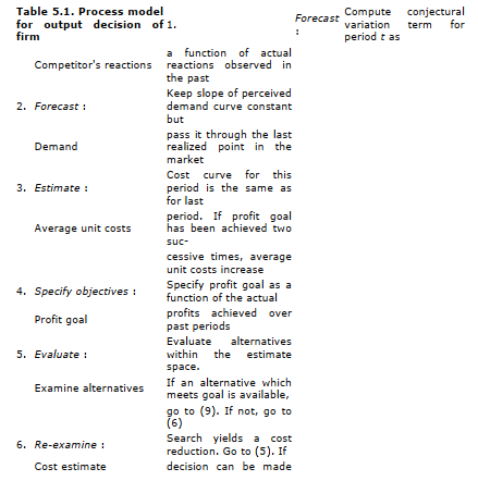
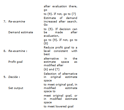
The decision-making process postulated by the theory begins with a forecast phase (in which competitor’s reaction, demand, and costs are estimated) and a goal specification phase (in which a profit goal is established). An evaluation phase follows, in which an effort is made to find the “best” alternative, given the forecasts. If this “best” alternative is inconsistent with the profit goal, a re-examination phase ensues, in which an effort is made to revise cost and demand estimates. If re- examination fails to yield a new best alternative consistent with the profit goal, the immediate profit goal is abandoned in favor of “doing the best possible under the circumstances.” The specific details of the models follow this framework.

Forecasting competitor’s behavior. Since we deal with a duopoly, one of the significant variables in the decision on the quantity of output to produce for each firm becomes an estimate of the rival firm’s output. For example, assume the monopolist in period t is considering a change in output from period ( t – 1) and makes an estimate of the change the splinter will make. At the end of period t the monopolist can look back and determine the amount of change the splinter made in relation to his own change. The ratio of changes can be expressed as follows:

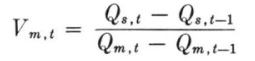
where V _m,t = the change in the splinter’s output during period  t as a proportion of the monopolist’s output change during period t, Q _s,t – Q _{s,t – 1} = the actual change in the splinter’s output during period t, Q _m,t – Q _m,t-1, = the actual change in the monopolist’s output during period t.

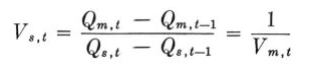
In the same way we have for the splinter the following:

We assume that the monopolist first makes an estimate of the fractional change in the splinter’s output in relation to his own change, that is, an estimate of V _m,t. We have assumed that the monopolist will make this estimate on the basis of the splinter’s behavior over the past three time periods. More specifically, we have assumed that the monopolist’s estimate is based on a weighted average, as follows:

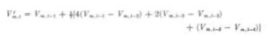
where V ′ _m,t = the monopolist’s estimate of the change in the splinter’s output during period t as a proportion of the monopolist’s output change during period t, that is, an estimate of V _m,t •

Note that ( V′ _m,t) •( Q _m,t – Q, _{m t-1} ) is the monopolist’s estimate of the splinter’s change in output, Q, _{s t} – Q, _{s t minus;1} •

We would expect the splinter firm to be more responsive to recent shifts in its competitor’s behavior and less attentive to ancient history than the monopolist, both because it is more inclined to consider the monopolist a key part of its environment and because it will generally have less computational capacity as an organization to process and update the information necessary to deal with more complicated rules. Our assumption is that the splinter will simply use the information from the last two periods. Thus,

In the same manner as above, ( V′ _s,t )•( Q _s,t – Q _s,t-1 ) is the splinter’s estimate of the monopolist’s change in output, Q _m,t – Q _m,t-1.

Forecasting demand. We assume that the actual market demand curve is linear. That is, we assume the market price to be a linear function of the total output offered by the two firms together. We also assume that the firms forecast a linear market demand curve (not necessarily the same as the actual demand curve). There has been considerable discussion in the economics literature of an alleged discrepancy between the “imagined” demand curve and the actual demand curve, and it is this concept that is incorporated in the model. The values of the parameters of the imagined demand curve are based on rough inferences from the nature of the firms involved.

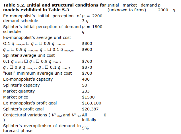
We assume that, because of its past history of dominance and monopoly, the ex- monopolist will be overly pessimistic with respect to the quantity that it can sell at lower prices, i.e., we assume the initially perceived demand curve will have a somewhat steeper slope than will the actual market demand curve. On the assumption that information about actual demand is used to improve its estimate, we assume that the monopolist changes its demand estimate on the basis of experience in the market. The firm assumes that its estimate of the slope of the demand curve is correct and it repositions its previous estimate to pass through the observed demand point.

We posit that the splinter firm will initially be more optimistic with respect to the quantity that it can sell at low prices than the  ex-monopolist. Secondly, we assume that initially the splinter firm perceives demand as increasing over time. Thus, until demand shows a downward turn, the splinter firm estimates its demand to be 5 per cent greater than that found by repositioning its perceived demand through the last point observed in the marketplace.

Estimating costs. We do not assume that the firm has achieved optimum costs. We assume, rather, that the firm has a simplified estimate of its average cost curve, that is, the curve expressing cost as a function of output. It is horizontal over most of the range of possible outputs; at high and low outputs (relative to capacity) costs are perceived to be somewhat higher.

Further, we make the assumption that these cost estimates are “selfconfirming,” i.e., the estimated costs will, in fact, become the actual perunit cost. The concept of organizational slack as it affects costs is introduced at this point. Average unit cost for the present period is estimated to be the same as the last period, but if the profit goal of the firm has been achieved for two consecutive time periods, then costs are estimated to be 5 per cent higher than “last time.” The specific values for costs are arbitrary.

The monopolist’s initial average unit cost is assumed to be $800 per unit in the range of outputs from 10 to 90 per cent of capacity. Below 10 per cent and above 90 per cent the initial average unit cost is assumed to be $900.

It is assumed that the splinter will have somewhat lower initial costs. This is because its plant and equipment will tend to be newer and its production methods more modern. Specifically, initial average costs are $760 in the range of outputs from 10 to 90 per cent of capacity. Below 10 per cent and above 90 per cent costs are assumed to average $870 per unit produced.

Specifying objectives. The multiplicity of organizational objectives is a fact with which we deal in later models. For the present, however, we limit ourselves to a single objective defined in terms of profit. In this model the function of the profit objective is to restrict or encourage search as well as to determine the decision. If, given the estimates of rival’s output, demand, and cost, there exists a production level that will provide a profit that is satisfactory, we assume the firm will produce at that level. If there is more than one satisfactory alternative, the firm will adopt that quantity level that maximizes profit.

We assume that the monopolist, because of its size, substantial  computational ability, and established procedures for dealing with a stable rather than a highly unstable environment, will tend to maintain a relatively stable profit objective. We assume that the objective will be the moving average of the realized profit over the last ten time periods. Initially, of course, the monopolist will seek to maintain the profit level achieved during its monopoly.

The splinter firm will presumably be (for reasons indicated earlier) inclined  to consider a somewhat shorter period of past experience. We assume that the profit objective of the splinter will be the average of experienced profit over the past five time periods and that the initial profit objective will be linked to the experience of the monopolist and the relative capacities of the two. Thus, we specify that the initial profit objectives of the two firms will be proportional to their initial capacities.

Re-examination of costs. We assume that when the original forecasts define a satisfactory plan, there will be no further examination of them. If, however, such a plan is not obtained, we assume an effort to achieve a satisfactory plan in the first instance by reviewing estimates and finally by revising objectives. We assume that cost estimates are reviewed before demand estimates and that the latter are only re- examined if a satisfactory plan cannot be developed by the revision of the former. The re-evaluation of costs is a search for methods of accomplishing objectives at lower cost than appeared possible under less pressure. We believe this ability to revise estimates when forced to do so is characteristic of organizational decision making. It is, of course, closely related to the organizational slack concept previously introduced. In general, we have argued that an organization can ordinarily find possible cost reductions if forced to do so and that the amount of the reductions will be a function of the amount of slack in the organization.

It is assumed that the re-examination of costs under the pressure of trying to meet objectives enables each of the organizations to move in the direction of the “real” minimum cost point. For purposes of this model it is assumed that both firms reduce costs 10 per cent of the difference between their estimated average unit costs and the “real” minimum.

Re-examination of demand. The re-evaluation of demand serves the same function as the re-evaluation of costs. In the present model it occurs only if the re-evaluation of costs is not adequate to define an acceptable plan. It consists of revising upward the expectations of market demand. The reasoning is that some new alternative is selected that the firm believes will increase its demand. The new approach may be changed advertising procedure, a scheme to work salesmen harder, or some other alternative that leads the firm to an increase in optimism. In any event, it is felt the more experienced firm will take a slightly less sanguine view of what is possible. As in the case of estimating demand, we assume that all firms persist in seeing a linear demand curve and that no changes are made in the perceived slope of that curve. In the case of the ex-monopolist, it is assumed that as a result of the re-examination of demand estimates, the firm revises its estimates of demand upward by 10 per cent. In the case of the splinter, the assumption is that the upward revision of demand is 15 per cent.

Re-examination of objectives. Because our decision rule is one that  maximizes among the available alternatives and our rule for specifying objectives depends only on outcomes, the re-evaluation of objectives does not, in fact, enter into our present models in a way that influences behavior. The procedure can be interpreted as adjusting aspirations to the “best possible under the circumstances.” If our decision rule were different or if we made (as we do in later chapters) objectives at one time period a function of both outcomes and previous objectives, the re-evaluation of objectives would become important to the decision process.

Decision. We have specified that the organization will follow  traditional economic rules for maximization with respect to its perception of costs, demand, and competitor’s behavior. The specific alternatives selected, of course, depend on the point at which this step is invoked (i.e., how many re-evaluation steps are used before an acceptable plan is identified). The output decision is constrained in two ways:

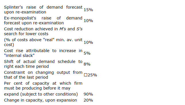
1. A firm cannot produce, in any time period, beyond its present capacity. Both models allow for change in plant capacity over time. The process by which capacity changes is the same for both If profit goals have been met for two successive periods and production is above 90 per cent of capacity, then capacity increases 20 per cent.
2. A firm cannot change its output from one time period to the next more than □25 per The rationale behind the latter assumption is that neither large cutbacks nor large advances in production are possible in the very short run, since there are large organization problems connected with either.

The various initial conditions specified above are summarized in Table 5.2, along with the other initial conditions required to program the models.

3. RESULTS   OF   THE   DUOPOLY MODEL

We have now described a decision-making model of a large ex-monopolist and a splinter competitor. In order to present some detail of the behavior that is generated by the interacting models, we have reproduced in Table 5.3 the values of the critical variables on each of the major decision and output factors. By following this chart over time, we can determine the time path of such variables as cost, conjectural variation, and output for both of the firms.

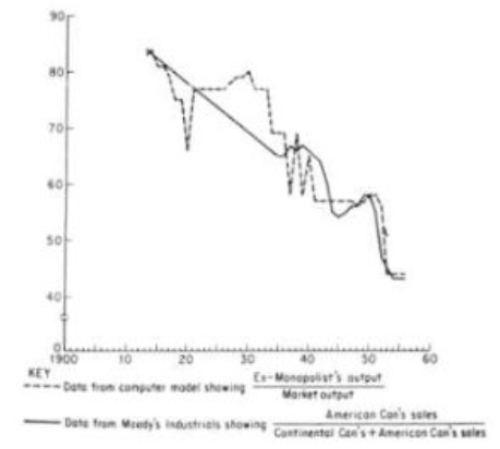
Figure 5.1 Comparison of share of market data.

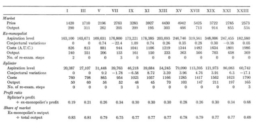
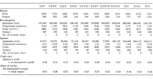
Table 5.3. Values of selected variables at two-period intervals

In addition, we have compared the share of market and profit-ratio results with actual data generated from the competition between American Can Company and its splinter competitor, Continental Can Company, over the period from 1913 to 1956. These comparisons are indicated in Figs. 5.1 and 5.2. In general, we feel that the fit of the behavioral model to the data is surprisingly good, although we do not regard this fit as validating the approach. It should be noted that the results in period XLV do not necessarily represent an equilibrium position. By allowing the firms to continue to make decisions, changes in output as well as changes in share of market would result. One of the reasons for the expected change is that the demand curve is shifting upward. Another more interesting reason is that no changes have been made within the organizations. In particular, the splinter firm is a mature firm by period XLV, but in the model it behaves as a new, young firm.An examination of Table 5.3 indicates that the re-examination phase of the decision- making process was not used frequently by either firm. This characteristic is the result of a demand function that is increasing over most of the periods. Whether this also stems from an inadequacy in the model’s description of organizational goal setting or is a characteristic of the real world of business decision making is a question that can be answered only by empirical research.

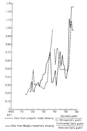
Figure 5.2 Comparison of profit-ratio data.

4. Deficiencies

The results of the model indicate that it is feasible to construct a choice model based on the general concepts outlined in Chapters 3 and 4. The theory we have used differs from conventional theory in six important respects:

1. The models are built on a description of the decision process. That is, they specify organizations that evaluate competitors, costs, and demand in the light of their own objectives and (if necessary) re-examine each of these to arrive at a decision.
2. The models depend on a theory of search as well as a theory of choice.
3. They specify under what conditions search will be intensified (e.g., when a satisfactory alternative is not available). They also specify the direction in which search is undertaken. In general, we predict that a firm will look first for new alternatives or new information in the area it views as most under its control. Thus, in the present models we have made the specific prediction that cost estimates will be re-examined first, demand estimates second,  and organizational objectives third.

3. The models describe organizations in which the profit objective changes over time as a result of experience. The goal is not taken as given initially and fixed It changes as the organization observes its success (or lack of it) in the market. In these models the profit objective at a given time is an average of achieved profit over a number of past periods. The number of past periods considered by the firm varies from firm to firm.
4. Similarly, the models describe organizations that adjust forecasts on the basis of Adaptation in expectations occurs as a result of observations of actual competitors’ behavior, actual market demand, and actual costs. Each of the organizations we have used readjusts its perceptions on the basis of such experience.
5. The models introduce organizational biases in making estimates. For a variety of reasons we expect some organizations to be more conservative with respect to cost estimates than other organizations, some organizations to be more optimistic with respect to demand, and some organizations to be more attentive to and perceptive of changes in competitors’ plans.
6. The models all introduce features of “organizational slack.” That is, we expect that over a period of time during which an organization is achieving its goals, a certain amount of the resources of the organization are funneled into the satisfaction of individual and subgroup objectives. This slack then becomes a reservoir of potential economies when satisfactory plans are more difficult to choice.

Despite the substantial differences between the duopoly model and more classical models in this area, a number of important features of organizational decision making as we have observed it are omitted from the model. In particular, we would identify the following major ways in which the model is deficient as a description of the choice process in a modern firm:

1. Price is not a decision variable. In order to simplify the model, we have made a single decision variable (output) rather than a series of decision variables — including price.
2. Only one goal is considered. A more complete model would include more than a single goal.
3. Little explicit attention is given to standard operating procedures and the avoidance of uncertainty through substituting feedback data for expectational data.

4. The organizations learn from their environment in only a limited sense. Decisions are contingent on feedback but decision rules are not.

These deficiencies suggest that the duopoly model, despite its apparent success, is not a general model. Thus, we need to consider in somewhat more detail the actual procedures used by business firms to make economic decisions. We will argue that business firms adapt over time by learning a number of simple decision rules and procedures and that a behavioral theory of the firm should deal both with that adaptive process and with the procedural implications of long-run adaptation.

Source: Skyttner Lars (2006), General Systems Theory: Problems, Perspectives, Practice, Wspc, 2nd Edition.