The general model presented in this chapter is a summary of our understanding of the key microprocesses in price and output determination by a modern firm. It is a framework for other models and a basis for exploring the reaction of such firms to characteristics of the market, variations in external (e.g., governmental) constraints, and other conventional economic questions. As a prelude to such theoretical efforts and to attempts to test the model, we have undertaken an examination of some basic properties of the model. In this section we discuss the results of the first stage of that examination.

1.  A    MULTIPLE    REGRESSION PROCEDURE FOR ANALYSIS

We wish to determine the extent to which behavior in the model is sensitive to variations in various internal parameters. ³ An exhaustive consideration of that question is not really feasible. The number of outputs and the number and combinations of inputs are of an intolerable order of magnitude from the point of view of complete analysis. The model generates a detailed time series of decisions, internal organizational results, goals, and so on for each firm in the industry. As we have already noted, it depends on a rather large number of initial conditions and parameters.

To make the analysis we limited attention to a few summary statistics of key output variables and to a sample of parameter inputs. The choice of output to consider and the constraints on the parameter sample were made on the basis of a priori judgments on importance and probable sensitivities. Within those constraints, the specific samples to be considered were determined randomly.

Industry and market simplifications. To study the impact of selected internal firm parameters on the model, we have simplified the industry by treating only the two-firm case. There are two firms in the industry, competing in the same market. There are no product differences between the two firms. In addition, we consider only one set of market parameters and a market in which the exogenous factor contributing to total demand ( EXT ) is subject only to modest random fluctuations around the mean. Values used for the market parameters and initial conditions are shown in Table 8. 1. EXT was normally distributed with a mean 1.0 and a standard deviation 0.1. Values of EXT were serially independent and are listed in Table 8.2.

Output variables. For each of the two firms, we computed means of four different variables over three different time spans. Thus, we limited ourselves to 24 output variables. The four variables chosen were four common economic variables involved in the model — price, inventory, market share, and profit. The analysis considered the sensitivity of those variables to changes in internal parameter values. The time spans chosen were the last five time periods of the series, the last ten time periods of the series, and the last 25 time periods of the series. The total series consisted of 50 time periods. A complete listing of the output variables used in the analysis and their variable names in the computer program are indicated in Table 8.3.

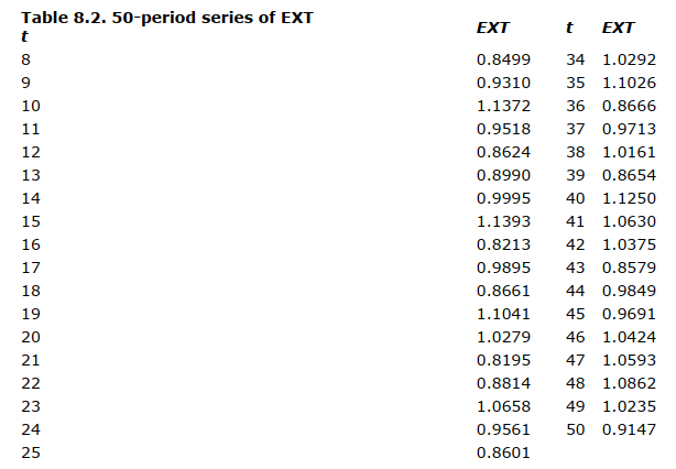
Table 8.3. Output variables and program names

Fixed internal parameter values. To simplify the analysis further, we held a substantial number of parameter values constant. In fact, we limited variation to 25 internal parameters and initial values. The number 25 was determined largely by technical requirements. The specific parameters and initial values that were  kept fixed were chosen on the basis of two simple criteria. First, we fixed the parameters for one of the two firms. This “fixed” firm was the same (with respect to the values assigned to its parameters and initial conditions) throughout the analysis. The second, or “variable,” firm had different values for 25 internal parameters and initial conditions. Of these 25 independent variables, five were initial conditions and 20 were parameters. We attempted to choose those variables that seemed a priori most likely to be important to the operation of the model. In practice, this meant that we included virtually every variable within the model that had direct effect on the decision variables, on adaptation of those decision variables, or on adaptation in goals. Table 8.4 gives the complete list of the parameters and initial conditions that were fixed for the two firms and the values assigned to each. Variable internal parameters and sampling procedures. The 25 independent variables of the analysis defined a parameter space from which we wished to sample in order to test the effects of changes in parameter values. Our analysis is based on a sample of size 100 drawn from this parameter space in the following way:

1. For each parameter we determined a mean value, a range, and a In each case the mean value was also the value assigned to the fixed firm for the same parameter. The range was designed to restrict possible variations in parameter values to a more or less reasonable extent. The distribution could be either approximately normal or approximately rectangular.

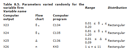
2. From these distributions of parameter values we drew 100 random values for each of the 25 values. In effect, we created 100 different “firms” by a random combination of parameter values. The 25 variable names (in three forms — flow chart, internal computer program, and computer output), the ranges assigned, and the form of the distribution are indicated in Table 8.5. A check on the parameter values actually generated by the program indicates that the program did, in fact, choose values consistent with the specifications of range and form of distribution.

Variations in the analysis. Within the model we have not specified whether sales and market share goals are in terms of sales revenue or in terms of product units sold. By varying that aspect of the model, we have obtained three  different variations of the basic model each of which has been analyzed. In Variation I sales goals are in terms of revenue, and market share goals are in terms of share of the revenue. In Variation II, sales goals are in terms of product units but market share goals are in terms of share of revenue. In Variation III, sales goals are in terms of product units and market share goals are in terms of share of the product units sold.

Basic procedures of analysis. The simplification of the model permits an analysis of the following sort: we have 24 dependent variables. For each of these variables we have 25 independent variables and 100 observations of the model. This situation is repeated in each of the three variations of the model. To these data we apply a multiple regression model to determine (within the linear constraints of that model) the contribution of variations in the parameter values to variations in the output. The multiple regression procedure adds and drops variables systematically (reconsidering the entire set of variables at each stage) according to their contribution to the F -values associated with the regression. It identifies all variables that meet an arbitrary criterion of contribution, the criterion being the same for all 24 regression analyses.

These procedures, although somewhat complex, are also certainly somewhat crude. They involve a host of assumptions both in the simplifications and in the use of multiple regression procedures. The multiple regression gives us only an occasional glimmer of potential interaction effects among the parameters, and we cannot be sure that the simplifications have not either concealed some important parameters or defined a specific market situation that leads to extreme results in the model. The model may behave quite differently under other reasonable initial conditions, under other market conditions, or under conditions in which there are more than two firms. Despite these obvious problems, the analysis has the virtue of feasibility. In retrospect, it also has the advantage that we have learned something from it. It has results, and the results seem to be meaningful.

2. Results of the analysis

The multiple regression analysis selects, for each output variable, those parameters to which the model is most consistently sensitive. We have identified about half of the original 25 parameters as being especially important. Parameters affecting the output of the variable firm. We will consider only those parameters to which the model is consistently sensitive in all three variations. Differences in sensitivity from one model variation to another do not seem to be particularly consistent. Among the 25 parameters and initial values considered, there are 11 that seem to have a consistent effect in one or two classes (i.e., price, inventory, market share, or profit) of output variables. There are three that have pervasive effects in three or four classes of variables.The parameters that have general effects are:

1. The proportional increase in the upper production limit when production is at full capacity (α ₈ ). The larger the value of this parameter, the faster the firm can adjust its production upward.
2. The extent of adjustment in price to competitive price changes or to required mark-up to maintain profitability (ß ₃ ). The larger the value of this parameter, the greater the reaction to competition and to apparently inadequate mark-up.
3. The initial propensity to modify price in reaction to failure on profit goals (ß ₅ ). The larger the value of this parameter, the greater the initial propensity to raise price.

The generality of the effect of these parameters seems to stem, at least in part, from some key characteristics of the market postulated for the model. Relative to the initial positions of the two firms, the market was substantially underexploited. As a result, most firms tended to raise price over time, and all firms expanded production. The parameters affecting the ease with which such adjustments were made had general effects. Such general effects would probably arise under a number of market conditions, but would not necessarily appear in all.

Aside from these pervasive influences, the output was primarily sensitive to the following parameters:

Price was affected by the parameters controlling increases ( a ₁ ) and decreases (α ₁₀) in slack, the amount of reduction feasible in sales promotion percentage (γ ₆ ), and the initial responsiveness of the profit goal to profit performance (ß ₂ ). In a general way, firms that had cost change alternatives to changes in price — that is, firms that could relatively easily vary slack, reduce promotion expenditures, and reduce profit goals — were likely to be relatively low-price firms in this market.

Inventory was affected by the rate at which the forecast of sales adjusted to past sales (α ₁₁ ). Compared with its performance elsewhere, the multiple regression model did not do an especially good job of predicting inventory levels.

Market share was affected primarily by the parameters controlling the upward adjustment of sales effectiveness pressure ( c ₁ ) and the upward (γ ₄ )  and downward (γ ₆ ) adjustment of sales promotion percentage.

Profit was affected primarily by the parameters controlling the initial rate of adjustment of sales goals to sales results (γ ₁ ) and those controlling second-order learning of adjustment parameters (η, Δ).

The pattern of sensitivity to parameters is shown in Table 8.6.

Parameters affecting the output of the fixed firm. For obvious reasons, the analysis of the output of the fixed firm is less interesting immediately and somewhat less easy to understand. The direct parameter effects in the model are prima facie effects on the variable firm. The analysis of their effects on the fixed firm presupposes a detectable interaction between the firms. The parameters affecting price, inventory, and profit levels are indicated in Table 8.7. The market share analysis, of course, is identical to the previous market share analysis in a two-firm industry.

8.1.3    Implications of the analysis

On the whole, the multiple regression analysis confirms our intuitions about the model. In particular, we see five major implications:

1. The behavior of the model is partially dependent on the interaction between one set of internal parameters and the attributes of the market within which the model operates. Both the amount and direction of price change and changes in feasible production are controlled by certain key parameters that become important as the market conditions induce pressure for the decision rule involved to be used. For example, if demand induces a pressure for an increased upper production limit or for a decreased lower production limit, the magnitude of the shift is dictated by a specific parameter in the model.

2. The output of the model is substantially independent of a number of parameters affecting adjustments within the inventory-output Rates of adjustments in proposed inventory, runout level, and excess level (α ₁, α ₂, α ₃, α₄, α ₅, α ₆ ) apparently do not have a major impact, nor does the number of periods of history maintained on production level (π), although this may be a special function of the fact that the market tended to expand in the cases examined.

3. Most of the parameters to which the model is sensitive have relatively localized effects on certain classes of outputs. The pairings are about what might be suspected from an inspection of the structure of the model. Price is especially sensitive to cost parameters since price is associated with profit goals and achievement of profit goals involves in part the maintenance of an appropriate cost-price spread. Market share is especially sensitive to the decision variables (sales effectiveness pressure and sales promotion percentage) in the sales area and, thus, is especially sensitive to the parameters influencing changes in those decisions.
4. Profit seems to be especially sensitive to learning parameters (η, Δ). These parameters, affecting the adaptation in other adjustment mechanisms, are logically the most “fundamental” parameters of the model. Their influence on performance (in terms of the multiple regression analysis) is most pronounced with respect to profit.
5. It is not yet obvious that a dramatic reduction in the number of parameters in the model can be achieved by sensitivity analysis of this type. We have focused attention on about half of the original 25 parameters introduced for examination. We probably cannot reduce the number further so long as the model is in its present form. We may have to expand the number as we experiment with different market conditions and investigate some of the parameters and initial conditions rejected for a priori reasons in this analysis.

As we mentioned earlier, the model presented in this chapter is basically a report on the first stage of a research program. The analysis presented here was designed to facilitate two additional steps in that research program — more detailed investigation of parameter effects and a study of the empirical implications of the model. Both of these additional steps need to be taken, and both can be accomplished more effectively on the basis of the present analysis. With respect to the empirical investigation, one of the problems with the model is the need to observe directly or to estimate a rather large number of parameters. As we reduce the number of critical parameters to a dozen or so, we can begin to see a feasible testing procedure. With respect to a more detailed study of one part of the parameter space, it is clear that an important next step is to consider more intensively the reaction of the model to the parameters identified in the present analysis.

Source: Skyttner Lars (2006), General Systems Theory: Problems, Perspectives, Practice, Wspc, 2nd Edition.