The separability in transfer and effort of the agent’s utility function simplifies the principal-agent theory with moral hazard by ensuring that the agent’s participation constraint is binding. However, it neglects one significant incentive effect, namely that one way to provide incentives is to make the agents richer by decreasing their marginal disutility of effort. The interaction between consumption and effort is clearly important in development economics when one wants to study agrarian contracts. For example, richer agents may be able to have a better diet, which increases their resistance. Then, the optimal compensation may entail a fixed payment whose objective is to bring the agent to a utility level where the marginal disutility of effort is lower. This type of compensation may require leaving him a rent which has a different (even though related) motivation than the limited liability rent exhibited in chapter 4.
In section 5.3.1, we show graphically how nonseparability calls for relaxing the participation constraint. Nevertheless, section 5.3.2 provides an example without wealth effect where the nonseparability is not exploited by the principal to relax the participation constraint.
1. Nonbinding Participation Constraint
Let us now assume that the agent has a general utility function defined over transfers and effort, namely U = u(t, e). Contrary to the standard framework used so far, we no longer postulate a priori the separability between transfer and effort. Effort can still take either of two values e in {0, 1}; to simplify notations, let us denote u1(t) = u(t, 1) and u0(t) = u(t, 0). Because effort is costly, we obviously have u1(t) < u0(t) for all t. Moreover, for i in {0, 1}, ui(.) is still increasing and concave in t for all t (ui‘ > 0, ui” < 0).
For what follows, it is also interesting to denote the inverse function of u0(-) by h0(-), which is increasing and convex (h’0 > 0 and h0” > 0). Consider the case where u1(.) is a concave transformation of u0(-), i.e., u1(.) = g o u0(-) with g(-) increasing and concave. Intuitively, this means that exerting effort makes the agent more averse to monetary lotteries.
In this framework, incentive and participation constraints are written respec- tively as

Extending the methodology of chapter 4, we now introduce the following change of variables: ![]() . With these new variables, the incentive and participation constraints (5.76) and (5.77) are written respectively as
. With these new variables, the incentive and participation constraints (5.76) and (5.77) are written respectively as

The risk-neutral principal’s problem is thus written as

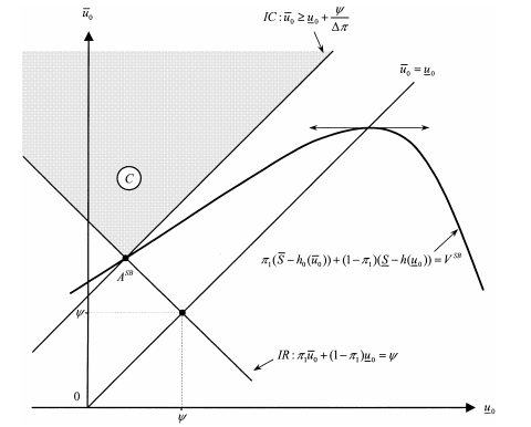
Figure 5.9: Solution in the Case of Separability
The fact that g(·) is concave ensures that the constrained set C of incentive feasible contracts ![]() is a nonempty convex set. Since the principal’s objec- tive function is strictly concave, the first-order Kuhn and Tucker conditions will again be necessary and sufficient to characterize the solution to this problem.
is a nonempty convex set. Since the principal’s objec- tive function is strictly concave, the first-order Kuhn and Tucker conditions will again be necessary and sufficient to characterize the solution to this problem.
Instead of proposing a general resolution to this problem, we restrict our- selves to a graphical description of the possible features of the solution for general functions u1(·) and u0(·) to satisfy the above properties. As a benchmark, it is use- ful to represent graphically the usual case of separability where, in fact, we have u1(t) = u0(t) − ψ for all t. In this case, we have immediately g(u) = u − ψ for all u, and u1(·) is simply a linear transformation of u0(·).
In figure 5.9, we have represented the set C of incentive feasible contracts in the case of a separable utility function. It is a dieder turned downward and lying strictly above the 45◦ line. The principal’s indifference curve VSB is inversely U-shaped. It is graphically obvious that the optimal contract must therefore be on the extremal point ASB of the dieder. We easily recover our analytical result of section 4.4. The risk-averse agent receives less than full insurance at the opti- mum, and the agent’s participation constraint is also binding.
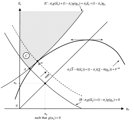
Figure 5.10: Solution in the Case of Nonseparability
Let us now turn to the case of nonseparability, which is the focus of this section. Figure 5.10 represents the set C of incentive feasible contracts and the possible second-best optimal contract A.
With a nonseparability, the binding incentive constraint (5.78) defines a locus of contracts that is no longer a straight line but a strictly convex curve in the plan ![]()
Similarly, the binding participation constraint (5.79) also defines a convex locus. The set C of incentive feasible contracts is again strictly convex, with an extremal point A still obtained when both constraints are binding. However, the strict convexity of C now leaves some scope for the optimal contract to be at point BSB, where only the incentive constraint is binding. In this case, the best way to solve the incentive problem is to give up a strictly positive ex ante rent to the agent. This case is more likely to take place when the IC constraint defines a very convex curve, i.e., when g(·) is very concave. This occurs when the agent is much more risk averse when he exerts a positive effort than when he does not. In this case, offering a risky lottery to induce effort and keep the agent’s expected utility relatively low is costly for the principal. The principal prefers to raise the agent’s expected utility to move toward areas where a risky lottery is much less costly.
Remark: Before closing this section, let us notice that we have already presented in chapter 4 a simple example of a contracting environment where the agent’s participation constraint is slack at the optimum, that is when the risk-neutral agent is protected by limited liability.
2. A Specific Model with No Wealth Effect
Sometimes, even without any separability between transfer and effort in the agent’s utility function, the agent receives zero ex ante rent. For example, suppose that the agent’s cost of effort is counted in monetary terms. The agent’s utility function is no longer separable between income and effort, and it is written as uft − efegg, where uf·g is again increasing and concave. With our usual notations, the moral hazard incentive constraint is now written as
![]()
The participation constraint is now
![]()
where u(0) is the agent’s reservation utility that he obtains when he refuses the contract.
Let us also assume that the agent has a constant risk aversion, namely the constant absolute risk aversion (CARA) utility function u(x) = − exp(−rx). When facing a binary lottery yielding wealths a and b with respective probabilities π and 1 − π, this agent obtains a certainty equivalent of income, which is defined as
![]()
where ![]() is a risk premium.
is a risk premium.
One can check that cfli xg is increasing with x for all x ≥ 0.
Using this formulation based on certainty equivalents, we can now rewrite (5.80) and (5.81) as

The principal’s problem becomes:

It is important to note that these constraints depend in a separable way on, first, the average transfer ![]() received by the agent and, second, the risk created by these transfers
received by the agent and, second, the risk created by these transfers ![]() . More precisely, the principal can ensure that the participation constraint (5.84) is binding by reducing the agent’s average transfer without perturbing the power of the incentive contract, i.e., still keeping the incentive constraint (5.83) satisfied. Indeed, this latter constraint can also be written as
. More precisely, the principal can ensure that the participation constraint (5.84) is binding by reducing the agent’s average transfer without perturbing the power of the incentive contract, i.e., still keeping the incentive constraint (5.83) satisfied. Indeed, this latter constraint can also be written as
![]()
where ![]() is the incentive power of the contract. We leave it to the reader to check that this incentive constraint must be binding. The second-best power of incentives ΔtSB is thus the unique positive solution to
is the incentive power of the contract. We leave it to the reader to check that this incentive constraint must be binding. The second-best power of incentives ΔtSB is thus the unique positive solution to
![]()
Given that the participation constraint (5.84) is also binding, the optimal second-best transfers are defined by:

By inducing effort, the principal therefore gets
![]()
If he does not induce effort, the principal can offer ![]() . The principal thereby gets an expected payoff
. The principal thereby gets an expected payoff ![]() . Hence, the principal prefers to induce effort when
. Hence, the principal prefers to induce effort when ![]() . Under complete information, the principal induces a first-best effort by offering a constant wage t¯ = t = ψ, and the optimal effort is positive when ΔπΔS ≥ ψ.
. Under complete information, the principal induces a first-best effort by offering a constant wage t¯ = t = ψ, and the optimal effort is positive when ΔπΔS ≥ ψ.
Therefore, as in a model with separability between consumption and effort, the principal induces a positive effort less often than in the first-best world, because ![]() is strictly positive when ΔtSB > 0.
is strictly positive when ΔtSB > 0.
Source: Laffont Jean-Jacques, Martimort David (2002), The Theory of Incentives: The Principal-Agent Model, Princeton University Press.