Initially attributed to German political economist Karl Marx (1818-1883) but later revised by, among others, Polish-born engineer and economist Michal Kalecki (1899-1970); political business cycle attributes economic fluctuations to politicians who manipulate fiscal and monetary policies (choosing between employment or inflation) in order to get elected/re-elected.
It is argued that in the period leading up to an election, policies are introduced to reduce unemployment regardless of the inflation which may result; however, after a successful election the party will introduce deflationary policies.
This throws the economy into disequilibrium. Kalecki argued that big business is opposed to government experiments to create full employment through spending (as seen in the Depression of the 1930s in every country except Nazi Germany).
Their dislike stems from a distrust of government interference in employment, a dislike of the areas in which spending is directed (public investment and subsidized consumption), and a dislike of the social and political changes arising from the creation of full employment.
Also see: business cycle, Kondratieff cycles, sunspot theory, product life-cycle theory, acceleration principle, fine-tuning, multiplier accelerator, trade cycle
Source:
M Kalecki, ‘Political Aspects of Full Employment’, Political Quarterly, vol. XIV (October-December 1943), 322-31;
P Minford and D Peel, ‘The Political Theory of the Business Cycle’, European Economic Review, vol. x (1982), 252-70
Theory


The first systematic exposition of economic crises, in opposition to the existing theory of economic equilibrium, was the 1819 Nouveaux Principes d’économie politique by Jean Charles Léonard de Sismondi.[4] Prior to that point classical economics had either denied the existence of business cycles,[5] blamed them on external factors, notably war,[6] or only studied the long term. Sismondi found vindication in the Panic of 1825, which was the first unarguably international economic crisis, occurring in peacetime.[citation needed]
Sismondi and his contemporary Robert Owen, who expressed similar but less systematic thoughts in 1817 Report to the Committee of the Association for the Relief of the Manufacturing Poor, both identified the cause of economic cycles as overproduction and underconsumption, caused in particular by wealth inequality. They advocated government intervention and socialism, respectively, as the solution. This work did not generate interest among classical economists, though underconsumption theory developed as a heterodox branch in economics until being systematized in Keynesian economics in the 1930s.
Sismondi’s theory of periodic crises was developed into a theory of alternating cycles by Charles Dunoyer,[7] and similar theories, showing signs of influence by Sismondi, were developed by Johann Karl Rodbertus. Periodic crises in capitalism formed the basis of the theory of Karl Marx, who further claimed that these crises were increasing in severity and, on the basis of which, he predicted a communist revolution. Though only passing references in Das Kapital (1867) refer to crises, they were extensively discussed in Marx’s posthumously published books, particularly in Theories of Surplus Value. In Progress and Poverty (1879), Henry George focused on land’s role in crises – particularly land speculation – and proposed a single tax on land as a solution.
Classification by periods

Business cycle with it specific forces in four stages according to Malcolm C. Rorty, 1922
In 1860 French economist Clément Juglar first identified economic cycles 7 to 11 years long, although he cautiously did not claim any rigid regularity.[8] Later[when?], economist Joseph Schumpeter argued that a Juglar cycle has four stages:
- Expansion (increase in production and prices, low interest rates)
- Crisis (stock exchanges crash and multiple bankruptcies of firms occur)
- Recession (drops in prices and in output, high interest-rates)
- Recovery (stocks recover because of the fall in prices and incomes)
Schumpeter’s Juglar model associates recovery and prosperity with increases in productivity, consumer confidence, aggregate demand, and prices.
In the 20th century, Schumpeter and others proposed a typology of business cycles according to their periodicity, so that a number of particular cycles were named after their discoverers or proposers:[9]
 Proposed economic waves |
|
|---|---|
| Cycle/wave name | Period (years) |
| Kitchin cycle (inventory, e.g. pork cycle) | 3–5 |
| Juglar cycle (fixed investment) | 7–11 |
| Kuznets swing (infrastructural investment) | 15–25 |
| Kondratiev wave (technological basis) | 45–60 |
- The Kitchin inventory cycle of 3 to 5 years (after Joseph Kitchin)[10]
- The Juglar fixed-investment cycle of 7 to 11 years (often identified[by whom?] as “the” business cycle
- The Kuznets infrastructural investment cycle of 15 to 25 years (after Simon Kuznets – also called “building cycle”)
- The Kondratiev wave or long technological cycle of 45 to 60 years (after the Soviet economist Nikolai Kondratiev)[11]
Some say interest in the different typologies of cycles has waned since the development of modern macroeconomics, which gives little support to the idea of regular periodic cycles.[12]
Others, such as Dmitry Orlov, argue that simple compound interest mandates the cycling of monetary systems. Since 1960, World GDP has increased by fifty-nine times, and these multiples have not even kept up with annual inflation over the same period. Social Contract (freedoms and absence of social problems) collapses may be observed in nations where incomes are not kept in balance with cost-of-living over the timeline of the monetary system cycle.
The Bible (760 BCE) and Hammurabi’s Code (1763 BCE) both explain economic remediations for cyclic sixty-year recurring great depressions, via fiftieth-year Jubilee (biblical) debt and wealth resets[citation needed]. Thirty major debt forgiveness events are recorded in history including the debt forgiveness given to most European nations in the 1930s to 1954.[13]
Occurrence
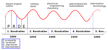
A simplified Kondratiev wave, with the theory that productivity enhancing innovations drive waves of economic growth
There were great increases in productivity, industrial production and real per capita product throughout the period from 1870 to 1890 that included the Long Depression and two other recessions.[14][15] There were also significant increases in productivity in the years leading up to the Great Depression. Both the Long and Great Depressions were characterized by overcapacity and market saturation.[16][17]
Over the period since the Industrial Revolution, technological progress has had a much larger effect on the economy than any fluctuations in credit or debt, the primary exception being the Great Depression, which caused a multi-year steep economic decline. The effect of technological progress can be seen by the purchasing power of an average hour’s work, which has grown from $3 in 1900 to $22 in 1990, measured in 2010 dollars.[18] There were similar increases in real wages during the 19th century. (See: Productivity improving technologies (historical).) A table of innovations and long cycles can be seen at: Kondratiev wave § Modern modifications of Kondratiev theory.
There were frequent crises in Europe and America in the 19th and first half of the 20th century, specifically the period 1815–1939. This period started from the end of the Napoleonic wars in 1815, which was immediately followed by the Post-Napoleonic depression in the United Kingdom (1815–30), and culminated in the Great Depression of 1929–39, which led into World War II. See Financial crisis: 19th century for listing and details. The first of these crises not associated with a war was the Panic of 1825.[19]
Business cycles in OECD countries after World War II were generally more restrained than the earlier business cycles. This was particularly true during the Golden Age of Capitalism (1945/50–1970s), and the period 1945–2008 did not experience a global downturn until the Late-2000s recession.[20] Economic stabilization policy using fiscal policy and monetary policy appeared to have dampened the worst excesses of business cycles, and automatic stabilization due to the aspects of the government’s budget also helped mitigate the cycle even without conscious action by policy-makers.[21]
In this period, the economic cycle – at least the problem of depressions – was twice declared dead. The first declaration was in the late 1960s, when the Phillips curve was seen as being able to steer the economy. However, this was followed by stagflation in the 1970s, which discredited the theory. The second declaration was in the early 2000s, following the stability and growth in the 1980s and 1990s in what came to be known as The Great Moderation. Notably, in 2003, Robert Lucas, in his presidential address to the American Economic Association, declared that the “central problem of depression-prevention [has] been solved, for all practical purposes.”[22] Unfortunately, this was followed by the 2008–2012 global recession.
Various regions have experienced prolonged depressions, most dramatically the economic crisis in former Eastern Bloc countries following the end of the Soviet Union in 1991. For several of these countries the period 1989–2010 has been an ongoing depression, with real income still lower than in 1989.[23] This has been attributed not to a cyclical pattern, but to a mismanaged transition from command economies to market economies.
a terrific file