The concept of output is not obviously relevant to a department store. In fact, if our major interest were in retail organizations, we would not describe any decisions as being output decisions. However, we are interested more generally in business firms, and we wish to identify a decision variable in the retail setting that has the same general attributes as the output decision in a production organization. A department store does not produce goods; it buys goods for resale. Consequently, orders and the process of making order decisions comprise the output determination of the firm. As the manufacturing firm adds to inventory by production, the retail firm adds to inventory by ordering.
As we have already suggested, the output decision is essentially a decision based on feedback from sales experience. No explicit calculation of the probable behavior of competitors is made, and although expectations with respect to sales are formed, every effort is made to avoid depending on any kind of long-run forecast. Output decisions are designed to satisfy two major goals. These are (1) to limit mark-downs to an acceptable level and (2) to maintain inventory at a reasonable level.
The firm divides output decisions into two classes — advance (initial) orders and reorders. Each is dependent on a different set of variables and performs a different function. Advance orders allow the firm (and its suppliers) to avoid uncertainty by providing contractual commitments. They also account for the bulk of the total orders. Reorders are only a small part of the total orders, but they provide virtually all the variance in total orders. Insofar as the output decision is viewed primarily as a decision with respect to total output, reorders are much more important than advance orders in fixing the absolute level.
1. Advance orders
Advance orders represent the base output of the department. The size of the advance order depends on two things: one is the estimated sales, the other a simple estimate of the variance in sales. In a general way, the apparent motivation with respect to advance orders is to set the commitment at such a level that the base output alone will be greater than sales only if extreme estimation errors have been made. Thus, refinements in estimation are not attempted and simple estimating procedures are used, modified somewhat by special organizational needs only remotely related to the issue of accuracy.
The estimation of sales. The store operates on a six-month planning period. The individual department estimates dollar sales expected during the next six months. At the same time, sales are estimated on a monthly basis for each product class over the six-month period. Since the accuracy of the estimate is not especially critical (at least within rather broad limits) for the total output decision, we consider the organizational setting in which the estimate is made in order to understand the decision rules. A low forecast, within limits, carries no penalties. The forecast cannot, however, be so low relative to past history that it is rejected (as being unrealistic) by top management. Limits on the high side are specified by two penalties for making a forecast that is not achieved. First, achievement of forecasts is one of the secondary criteria for judging the performance of the department. Although the department cannot significantly affect the sales goal by underestimation, it can to a limited extent soften criticism (for failure) by anticipating it. Second, an overestimate will result in overallocation of funds. If the department is unable to use the funds, it is subject to criticism. As a result, the sales estimate tends to be biased downward.
The primary data used in estimating sales are the dollar sales (at retail prices) for the corresponding period in the preceding year. Although the data are commonly adjusted slightly for “unique” events, the adjustments are not significant. The following naive rule predicts the estimates with substantial accuracy:
RULE 1. The estimate for the next six months is equal to the total of the corresponding six months of the previous year minus one-half of the sales achieved during the last month of the previous six-month period.
From the point of view of output decisions, the more critical estimates are those for the individual months. The monthly figures are used directly in determining advance orders for the individual seasons. The estimation procedure for a specific product class is as follows:
RULE 2. For the months of February, March, and April. Use the weekly sales of the seven weeks before Easter of the previous year as the estimate of the seven weeks before Easter of this year. In the same way, extend the sales of last year for the weeks before and after the season to the corresponding weeks of this year.
RULE 3. For the months of August and September. The same basic procedure as in Rule 2 is followed, with the date of the public schools’ opening replacing the position of Easter. The opening dates of county and parochial schools also are significant. If these dates are far enough apart, the peak will be reduced, but the estimate for the two months will still represent the total sales of the corresponding two months of the previous year.
RULE 4. For the months of May, June, October, November, and December. Estimated sales for this year equal last year’s actual sales.
RULE 5. For the months of January and July. Estimated sales for this year equal one- half of last year’s actual sales rounded to the nearest $100.
This set of simple rules provides an estimate of sales that is tightly linked to the experience of the immediately previous year with a slight downward adjustment (i.e., in Rule 5).
The seasonal advance order fraction. The department distinguishes four seasons — Easter, Summer, Fall, and Holiday. The seasons, in fact, do not account exhaustively for all months, but they account for most of the total sales. Estimates of sales are established on the basis of the monthly estimates. These estimates do not necessarily include all months in the season. The following estimation rules are used:
Easter: Cumulate sales for the seven weeks before Easter Summer: Cumulate sales for April, May, June, and one-half of July Fall: Cumulate sales for one-half of July,
August, and September Holiday: Cumulate sales for October, November, and December These cumulations give a seasonal sales estimate for use in establishing advance orders. Once such an estimate is made, some fraction of the estimated sales is ordered.
Advance orders generally offer some concrete advantages to the department. Greater selection is possible (some goods may not be available later), and some side payments may be offered by the producer (e.g., credit terms, extra services). The department exploits these advantages by ordering a substantial fraction of its anticipated sales in advance, but an attempt is made to limit the advance order fraction to an output that would be sold even under an extreme downward shift in demand.
The size of the advance order fraction is the result of learning on the part of the organization and reflects the differences among the seasons in sales variability and the degree of seasonal specialization of the items. The greater the susceptibility of seasonal sales to exogenous variables (e.g., weather), the lower the fraction. The more specialized the merchandise sold during a season (i.e., the greater the difficulty of carrying it over to another season), the lower the fraction. At the time we observed the organization, the fraction (estimated from interviews and analysis of data) and the timing of advance orders for each of the seasons were as follows:
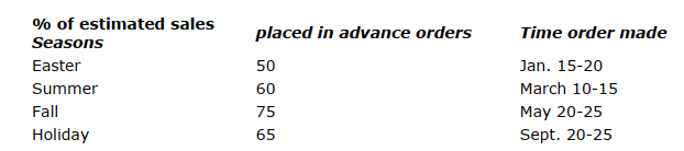
In general we expect this simple model to predict quite well, diverging only when the department makes ad hoc adjustments. Our observations lead us to believe this will not happen frequently.
2. Reorders
For all practical purposes, reorders control the total output of the department. As the word implies, a reorder is an order for merchandise made on the basis of feedback from inventory and sales. Because of leadtime problems, much of the feedback is based on early season sales information. Thus, the timing of a reorder depends on the length of time to the peak sales period as compared with the manufacturing lead-time required.
Reorder rules. Reorders are based on a re-estimate of probable sales. Data on current sales are used in a simple way to adjust “normal” sales. The reorder program specifies reorders for a given type of product class as a result of a simple algebraic adjustment.
Let T = the total period of the season r = the period of the season covered by the analysis S it = this year’s sales of product class i over r S ‘ ir = last year’s sales of product class i over r S ‘ i(T-r) = last year’s sales of product class i over T – r I i = available stock of i at time of analysis including stock ordered M i = minimum amount of stock of i desired at all times O i ( T-r ) = reorder estimate
Then,

If O i(T-r) ≤ 0 no reorders will be made. In addition, orders already placed may be canceled, prices may be lowered, or other measures taken to reduce the presumed overstocking. Such an analysis would be made for each product class. The figure that results is tentative, subject to minor modifications in the light of anticipated special events.
3. Open-to-buy constraint
The firm constrains the enthusiasms of its departments by maintaining a number of controls on output decisions. One of the more conspicuous controls is the “open-to- buy.” The open-to-buy is, in effect, the capital made available to each department for purchases. The open-to-buy for any month is calculated from the following equation:
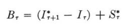
where B r = open-to-buy for month r I τ+1 = expected inventory (based on seasonal plans) for beginning of month ( r + 1) I τ = actual inventory at beginning of month τ Sτ = expected sales
The department starts each month with this calculated amount ( B τ ) minus any advance orders that have already been charged against the month. Any surplus or deficit from the preceding month will increase or decrease the current account, as will cancellation of back orders or stock price changes.
Although the open-to-buy is a constraint in output determination, it can be violated. As long as the preceding rules are followed and the environment stays more or less stable, the open-to-buy will rarely be exceeded. From this point of view, the open-to- buy is simply a long-run control device enforcing the standard reorder procedure and altering higher levels in the organization to significant deviations from such procedure. However, the constraint is flexible. It is possible for a department to have a negative open-to-buy (up to a limit of approximately average monthly sales). Negative values for the open-to-buy are tolerated when they can be justified in terms of special reasons for optimistic sales expectations.
The open-to-buy, thus, is less a constraint than a signal — to both higher management and the department — indicating a possible need for some sort of remedial action.
Source: Skyttner Lars (2006), General Systems Theory: Problems, Perspectives, Practice, Wspc, 2nd Edition.