In order to explore the effect of conflict (as reflected in presumed payoffs) on communicated information, we undertook two experiments on organizational communication. The first looks at individual bias, the second at organizational bias.
1. An experiment on communication bias
We wish to test the proposition that individuals can and do modify their subjective estimates of reality to accommodate their expectations about the kind of payoffs associated with various possible errors. In the experiment, subjects were asked to determine a summary statistic for an array of numbers. Since the experiment involved the switching of labels, it is of some importance to investigate the “theory” of descriptive statistics to determine the importance, if any, of the substantive origin of the numbers in the array to be summarized.
Essentially, a descriptive statistic is a procedure for transforming any arbitrary array of numbers into a coded number (or set of numbers) that in some sense “represents” the original array. The procedure is independent of the labels attached to the numbers in the original array. The arithmetic mean of the array {10, 8, 5, 1} is 6, and this result does not depend on whether we are talking about apples, revolutions per minute, or shoe size. According to the theory, the choice of a descriptive statistic (for example, a choice between an arithmetic mean and a median as a measure of central tendency) should be made on the basis of the characteristics of the distribution.
The implicit model underlying much of the treatment of descriptive statistics can be characterized as follows: For any array of numbers there exists a set of summary numbers (smaller in size than the original array) appropriate to that array. This set of summary numbers depends on the values of the numbers within the array and not on the labels attached to those numbers. Given an array of numbers and a set of instructions we can determine a statistic, and that statistic is uniquely defined, at least for any particular practitioner at any particular point of time.
Suppose, however, that the statistic is imbedded as an estimate in a decision-making system. In particular, suppose that the summary set of numbers represents information processed through an organization as a basis for a decision. We wish to investigate whether a summary estimate is uniquely determined for a given practitioner, a given array, and a given set of instructions. We do this by introducing variations in the labels attached to specific numbers in an array and comparing the summary statistic chosen by relatively sophisticated subjects.
In accordance with the model described above, it is hypothesized that cost analysts will tend to overestimate costs and that sales analysts will tend to underestimate sales. The rationale for the hypothesis relates to the presumption of a biased payoff schedule within the organization. The experiment described here does not test the rationale but only the treatment of the estimation problem.
Subjects. Subjects were 32 first-year graduate students in a program leading to a master’s degree in industrial administration. Almost all held undergraduate degrees in engineering or science; all were men; all had had some introduction to techniques of statistical description and estimation.
Experimental material. The basic experimental form was a paper-andpencil test requiring each subject to make ten estimates on the basis of the estimates of others. There were two versions of the test, the first of which (the cost version) was introduced by the following preamble:
Assume you are the chief cost analyst of a manufacturing concern considering the production of a new product. You have been asked to submit a single figure as your estimate of unit cost for the product if 750,000 are produced. You have two assistants (A and B) in each of whom you have equal confidence and who make preliminary estimates for you. For each of the cases below, indicate what estimate of cost you would submit.
The second version (the sales version) was introduced by the following preamble:
Assume you are the chief market analyst of a manufacturing concern considering the production of a new product. You have been asked to submit a single figure as your estimate of sales of the product if the price is set at $1.50. You have two assistants (A and B) in each of whom you have equal confidence and who make preliminary estimates for you. For each of the cases below, indicate what estimate of sales you would submit.
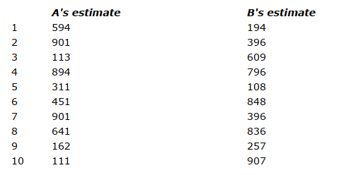
Each preamble was followed by a list of ten pairs of numbers representing the 10 pairs of estimates by two subordinates. These numbers and their pairings were identical in the two cases except that in the cost version they were presented as unit costs in cents and in the sales version they were presented as sales in 1000’s. The numbers ranged from 108 to 907. The pairs were arranged such that there were two pairs in which the difference was approximately 100, two pairs in which the difference was approximately 200, two pairs in which the difference was approximately 400, and two pairs in which the difference was approximately 500. For those eight pairs, one pair in each of the four difference levels was toward the high end of the over-all number range and one pair was toward the low end of the over- all range. The other two pairs did not fit the same pattern. One involved a difference of approximately 800; the other was simply a repeat of an earlier pair. The ten pairs in the order they were presented to the subjects are indicated below:
Experimental procedure. The subjects were divided into two groups of 16 subjects each. One group was given the cost version, the other the sales version. The two groups met in separate classes and completed the versions at approximately the same time without opportunity for communication. Ten weeks later the same groups were again given the forms. This time the versions were reversed. The group receiving the cost version first received the sales version ten weeks later. The group receiving the sales version first received the cost version ten weeks later. In all cases subjects were assured that the questions did not have a “correct” answer, that they should use their own best judgment, and that the test was not being used as an evaluative device.
Analysis. To analyze the data we define a number representing the weight attached to the larger of the two given numbers in the pair presented to the subject. We specify E = αU (1 – α)L, where E is the estimate made by the subject, U is the higher number in the pair, and L is the lower number in the pair. For each of the ten pairs for each subject, the value of a was computed as well as a mean a for the 10 pairs. The mean value of α represents the average weight attached to the higher of the two numbers in the given pair. Thus, a subject with α = 1 always chose the higher estimate; a subject with α = 0.50 on the average took the mean; a subject with a = 0 always chose the lower estimate. Since we have two estimates of α for each subject, we compare the a used in the cost version with the a used in the sales version. We treat the group that received the cost version first separately from the group that received the sales version first.
Results. The mean results for each group are indicated in Table 4.6.
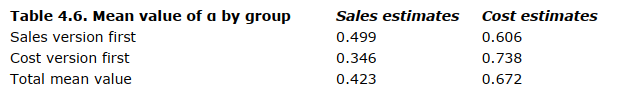
There is some suggestion in the data that the order of presentation might have affected the results. Therefore, before merging the two groups a test was run. Specifically, we tested the hypothesis that the two samples, sales version first and cost version first, came from the same population. The technique used was the Wald-Wolfowitz run test and the hypothesis was not rejected at the 5 per cent level of significance. The hypothesis that the total means are equal was then tested and the hypothesis was rejected.
A stronger test is one that utilizes the individual values. Specifically, we asked whether the value of a for a given subject was greater for the sales version, equal in the two versions, or greater in the cost version. The results for the 32 subjects are indicated in Table 4.7.
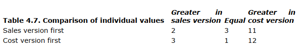
The results for both the sales version first and the cost version first are significant at the 0.05 level by the sign test.
In the most simplified terms, we can make the following generalizations from this study (and another to be discussed below): Individuals will treat estimates, information, and communication generally as active parts of their environment. They will tend to consider the decision for which the information is relevant, the probable outcomes of various possible biases in information, and the payoff to them of various possible decision results. They adjust the information they transmit in accordance with their perceptions of the decision situation.Such considerations led us in one early paper to develop some assumptions about the effect of communication structure (as well as some other attributes of the organization) on decision making. These assumptions formed the basis for a Cournot duopoly model in which the two firms had different communication structures and thus different biases. The result was a solution substantially different from that obtained in the conventional Cournot model. Subsequently, however, we have concluded that this approach was not fruitful. In the light of more recent research, it has two deficiencies as an approach to the study of organizational decision making.
- An approach that emphasizes expectations in the classic sense is inconsistent with our observations about how business organizations obtain and use information (see above). If, as we believe, organizations often substitute feedback mechanisms for anticipation data, models imputing bias in communication are more appropriately linked to the processing of feedback data than to anticipatory data.
- We cannot reasonably introduce the concept of communication bias without introducing its obvious corollary — “interpretive adjustment.” Those parts of the organization receiving data include human beings accustomed to the facts of communicative life. In short, they ordinarily use counterbiases to adjust for such biases as they anticipate in the data they receive.
The second deficiency represents an especially complex difficulty. Once we take the simple biases suggested by the study of the effect of labels on estimation and combine them in an organization, we compound the situation enough to make no simple model obviously appropriate. In order to study the organizational phenomena, we constructed a three-person experimental organization operating under a partial conflict of interest.
2. An experiment on organizational estimation under partial conflict of interest
The decision-making system in the experiment had four critical organizational characteristics:
- Subunit interdependence. Major decisions are not made by individuals or groups at the lowest level of the organization. Rather, the major decision-making units base their actions on estimates formulated at other points in the organization and transmitted to them in the form of communications. The estimates so received cannot be verified directly by the decision-making unit.
- Subunit specialization. The estimates used in decision making come from more or less independent subunits of the organization. Each such subunit specializes in a particular function and usually processes a particular type of information.
- Subunit discretion. Organizational constraints on the subunits that formulate and process estimates do not completely determine subunit The subunits have appreciable discretion in making, filtering, and relaying estimates.
- Subunit conflict. The freedom available to a subunit in satisfying organizational constraints is devoted to the satisfaction of subunit goals. Each subunit develops its own goals and procedures reflecting the particular interests of its members. Such subunit goals will be consistent with the organizational requirements, but within those limits they will take the direction most compatible with individual and group objectives.
Subjects. Subjects were 108 male students. They included both undergraduate and graduate students but were predominately undergraduate. Most of the subjects were either engineering or science majors. They were divided into 36 three-man groups.
Experimental situation: apparatus. Each member of a group sat in a booth designed to prevent him from seeing other members. Each subject was prevented from speaking to other members except when desired by the experimenter and then only over the communication system. This system provided each subject and the experimenter with a headset, microphone, and a display board that indicated what communication was currently feasible over the system. This system was controlled automatically by a mechanical timer which stepped the system through the various communication links required according to a predetermined schedule. When a particular subject was not currently able to use the communication system, a noise signal was transmitted over his line. This served both as a mask for room noise and as an auditory supplement to the visual display board signal.
Experimental situation: task. The task of the group was to estimate the area of a series of 30 rectangles. On each of the 30 trials, one member of the group (the length estimator) saw projected on the wall in front of him a line segment. The line segments varied in length from 2.27 to 4.92 in. There were 15 different lengths. The 15 were ordered randomly for presentation in the first 15 trials. The same lengths were presented in the last 15 trials (in a different random order). This line segment was designated as the length of the rectangle. It was not seen by the other two members of the group. A second member of the group (the width estimator) saw a different line segment projected on the wall in his booth. This line segment was designated as the width of the rectangle and was not seen by the other members of the group. The line segments were the same as for the length estimator and were presented in the same way but in a different random order. The third group member (the area estimator) received from the length estimator a number representing his estimate of the length. The area estimator received from the width estimator a number representing his estimate of the width. Neither the width estimator nor the length estimator heard the estimate of the other. The area estimator then communicated to the experimenter an estimate of the area of the rectangle. This estimate was compared with the correct area and the magnitude of the error was reported by the experimenter to all three group members. Aside from the communications indicated here, no communication among the members of the group was permitted.
Experimental situation: rewards. Each subject was given a card in his booth showing the basis on which he would be rewarded for the group’s performance during the experiment. The reward was in the form of cashconvertible points. The actual money involved was small (subjects normally “earned” about $1 in an experiment lasting about 40 minutes), but was adequate to obtain subjects. The major motivational factor was probably not the modest cash rewards but the point score. The experiment was presented as an experimental test for managerial potential, and most subjects reported after the experiment that they thought it measured some dimensions of managerial ability. There were three different payoff cards used in the experiment, as shown in Table 4.8.
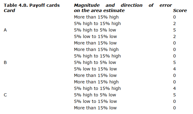
Each card indicated the highest payoff for estimates within 5 per cent of the true area. However, they differed in the extent to which they valued errors. Card A is symmetric around the true area. Card B suggests a preference for errors on the low side. Card C suggests a preference for errors on the high side. Subjects knew only their own payoff card. Experimental treatment. There were six different experimental treatments; in each treatment six groups were run. They were defined in terms of the assignment of payoff cards to the various members of the group. We will represent each treatment by three letters. The first letter is the payoff card given the length estimator; the second letter is the payoff card given the width estimator; the third letter is the payoff card given the area estimator.
AAA treatment. Each member of the group has the same payoff and it is symmetric.
BBB treatment. Each member of the group has the same payoff but it is not symmetric around the true area.
BCA treatment. The two line estimators have opposing biases and the area estimator has a symmetric payoff.
ACB treatment. All three payoffs are used. One of the line estimators has the symmetric payoff; the other two subjects have opposing biases.
CCB treatment. There are only biased payoffs. The two line estimators have the same bias and are opposed to the area estimator.
BCB treatment. There are only biased payoffs. One of the line estimators and the area estimator have the same bias. They are opposed by the other line estimator.
These six treatments represent six of the ten basic types of conflict possible in the experiment. That is, we feel that the following equivalences are reasonable:
BBB is equivalent to CCC.
ACB is equivalent to ABC, BAC, and CAB. BCA is equivalent to CBA.
CCB is equivalent to BBC.
BCB is equivalent to CBB, BCC, and CBC.
Unrepresented in the experiment are the following types: ABA (equivalent to ACA, BAA, and CAA), AAB (equivalent to AAC), ABB (equivalent to BAB, ACC, CAC), and BBA (equivalent to CCA).
Analysis. In the analysis we are primarily interested in the performance of the groups operating under the different conflict treatments. However, first we need to discuss the evidence bearing on the effectiveness of the experimental conditions in inducing consciously biasing behavior by subjects. Three pieces of evidence are available, none fully satisfactory. First, we compare the regression of estimates on actual line lengths for the three kinds of payoff cards used for line estimators. Second, we compare the values of d in the equation A = δ LW (where A is the area estimate, L is the length estimate, and W is the width estimate) for the two kinds of payoff cards (A and B) used for area estimators. Third, we compare the frequency of overt strategy comments indicating a conscious manipulation of estimates by individuals having biased payoff cards (B and C) as compared with persons having unbiased payoffs (A). The basic problem with all techniques is that the various individuals were involved in different kinds of groups such that it is impossible to make firm inferences as to the effect of the payoff cards on individual behavior independent of all group effects. These effects include both the pattern of payoffs to other participants and the local adaptation to area error.
To measure the performance of groups, we compute the mean absolute error and the mean algebraic error in estimating the area of the rectangle. Specifically, we consider the mean absolute and algebraic errors in estimating the area for each treatment for each of six five-trial periods.
Results. The regressions of estimated line segment length ( E ) on actual length ( L) for subjects having the various payoff cards have the following equations:
A (no bias): E = 3.28 + 1.05 ( L – 3.60)
B (low bias): E = 3.51 + 1.20 ( L – 3.60)
C (high bias): E = 3.65 + 1.19( L – 3.60)
The difference between the means is significant and in the predicted direction for the AC and the BC comparisons. The AB difference is significant but not in the predicted direction. The differences between the slopes of A and B and A and C are significant. The difference between the slopes of B and C is not significant. All tests were made at the 5 per cent level of significance.
The values of the “fudge factor,” δ, for the several area estimators are indicated below for each treatment:
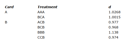
Subjects’ responses to a question eliciting comments on individual strategies were divided into those that showed some conscious biasing of subjective estimates and those that did not. Forty-four of the 78 subjects with biased payoffs expressed overtly such strategies. Nine of the 30 subjects with unbiased payoffs did so.
We conclude that the payoff cards did have the desired effect of introducing individual behavior directed toward biasing the organization estimate. The data in general support such a proposition.
The basic results with respect to the performance of the various groups are indicated in Fig. 4.1. We plot the mean absolute performance over each of the six five-trial periods for each treatment. Two things are conspicuous: (1) No treatment has any very clear advantage from the point of view of such performance. (2) There is an apparent convergence in performance over time.
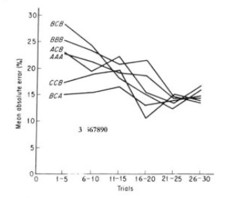
Figure 4.1
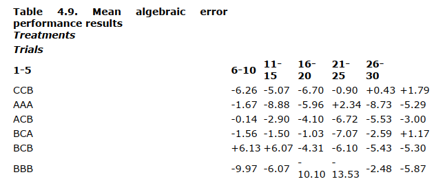
The results ( Table 4.9 ) with respect to algebraic error show no such consistency except for the treatment (BBB) involving bias without conflict. As might be expected, that treatment shows rather consistently the greatest negative error. The other five treatments are apparently indistinguishable (by Kendall’s test for concordance). There is a suggestion in the data for the final trials that net group bias may affect performance, but that result cannot be clearly distinguished from more transitory variations.
We conclude that there are no persistent differences among the performances of the groups that are a function of the extent or type of conflict imposed on them within this experiment.
The anomaly that variations in behavior at the micro level can exist actively without being reflected at a macro level is a common enough phenomenon. It does not elicit surprise after the fact. In the present situation we can understand how such a result might have been produced. In particular, it seems clear that in an organization of individuals having about the same intelligence, adaptation to the falsification of data occurs fast enough to maintain a more or less stable organizational performance. For the bulk of our subjects in both experiments, the idea that estimates communicated from other individuals should be taken at face value (or that their own estimates would be so taken) was not really viewed as reasonable. For every bias, there was a bias discount.
If such a result can be shown to be a general one, however, it has substantial implications for a theory of organizational decision making. We, as well as others, have argued that internal informational bias has to be dealt with explicitly in a theory of the firm. These results cast doubt on such an argument in extreme form. They indicate that such phenomena, important as they may be to the understanding of the internal operation of the organization, have a severely constrained significance to a theory of organizational choice.
The generality of such a result and such an implication, of course, needs to be explored further. However, our own experience in attempting to develop models of organizational price and output determination without explicit attention to internal information bias is consistent with the conclusion based on the experiment. Both because of the tendency toward counterbiasing and because of the relative unimportance of anticipatory data, we have been able to ignore such apparently important factors as communication effects on organizational expectations — at least in the development of the relatively frequent type of decision involved in determining price and output.
Source: Skyttner Lars (2006), General Systems Theory: Problems, Perspectives, Practice, Wspc, 2nd Edition.